
Stress Distribution Prediction in front of the crack tip using Artificial Neural Networks: A Data-Driven Approach in Fracture Mechanics
Downloads
Contents
Abstract
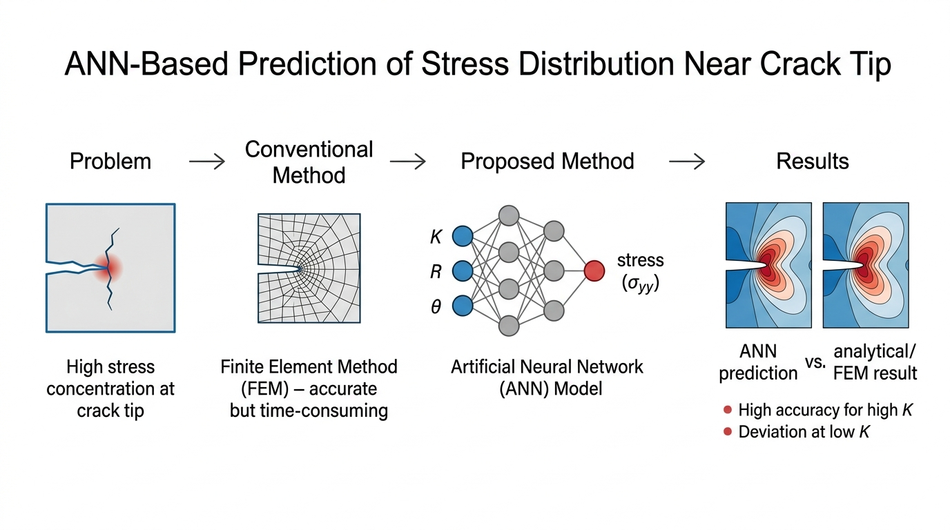
Understanding the stress distribution in front of the crack tip is essential because this region experiences high stress concentration that can control crack initiation and propagation. This study proposes an artificial neural network (ANN) model as a computationally efficient surrogate model for predicting the stress distribution and stress values in front of the crack tip in a simple cracked geometry. The proposed ANN model complements conventional finite element method (FEM) analyses by enabling rapid stress prediction once the model has been trained. The results show that the ANN model can capture the general relationship between the stress intensity factor, radial distance, angular position, and crack-tip stress. However, its predictive performance strongly depends on the magnitude of the stress intensity factor. At low K values, the ANN model shows significant discrepancies in both stress values and contour visualization, and it cannot accurately reproduce the theoretical butterfly-shaped stress distribution. At higher K values, the predicted stress distribution is closer to the analytical solution, and the contour shape is more consistent. These findings indicate that the present ANN model should be regarded as a proof-of-concept surrogate model with limitations, rather than a replacement for analytical LEFM solutions or FEM analysis.
Introduction
Engineers who build machines and structures will use design approaches to ensure safety, durability, and reliability. There are three design approaches, which are the material strength approach, the fracture mechanics approach, and the fatigue approach (Stephens et al., 2001; Anderson, 2017). In the material strength approach, the material-carrying load is assumed to be homogenous, continuum, and isotropic. This approach only compares the working stress in a component to the strength of the component material. Component materials are often found to contain a defect or flaw, such as a crack. The crack may cause a decrease in the strength of the material. Thus, the crack size must be taken into account to consider the load-carrying ability against material strength. The design approach that considers crack size and working stress is known as the fracture mechanics approach (Stephens et al., 2001; Anderson, 2017; Dowling et al., 2013). The previous cases are implemented in the design relating to static loads. A structure component rarely experiences static loads during its service. The structure almost entirely undergoes dynamic load. In this case, the design approach is the fatigue approach (Stephens et al., 2001; Dowling et al., 2013).
In the fatigue approach to design, the lifetime of a component can be predicted, and the remaining lifetime of a component can be estimated. There are four methods to estimate the lifetime of a component in the fatigue approach: stress-life (S-N), strain-life (ε-N), stress intensity factor-crack propagation rate (ΔK-da/dN), and the combined ε-N and ΔK-da/dN approaches (Stephens et al., 2001). The first and second methods are based on material strength, whereas the third method is based on fracture mechanics. In fracture mechanics, the stress concentration in front of the crack tip is a key parameter for evaluating structural integrity because it governs crack initiation and crack propagation. The crack-tip stress field can be estimated using analytical solutions derived from linear elastic fracture mechanics, while the finite element method (FEM) is widely used to calculate and visualize stress fields, crack-tip parameters, and plastic zone development around cracks (Tinoco et al., 2019; Tracey, 1971; Zhang et al., 2008; Chen et al., 2023; Mao et al., 2022; Prabaswara et al., 2023; Muflikhun et al., 2025). Previous FEM-based studies have demonstrated that numerical methods are effective for evaluating local stress concentration and crack-tip behaviour under various loading and material conditions. However, FEM implementation generally requires several computational steps, including geometry creation, material modeling, meshing, boundary condition definition, and numerical solution. The use of a large number of elements and nodes can also increase the computational time required to obtain accurate results (Logan, 2016). Therefore, ANNs provide a computationally efficient surrogate modeling approach that can complement FEM and analytical calculations in applications requiring rapid prediction.
Recent developments in machine learning have opened new opportunities for fracture mechanics analysis, particularly for problems involving complex stress/strain fields, crack-tip singularities, and computationally intensive numerical simulations. Artificial neural networks (ANNs) have been used for fatigue-crack growth prediction, fatigue life estimation, fatigue strength prediction, fretting fatigue life prediction, stress recovery in adaptive FEM, and fracture characterization from displacement data (Khaleghi et al., 2022; Khoei et al., 2020; Kazeruni & Ince, 2023; Ma et al., 2021; Barbosa et al., 2020; Nugroho et al., 2025). For example, Khaleghi et al. (2022) demonstrated that ANN-based approaches can be used for fracture characterization from noisy displacement fields, showing the potential of neural networks to extract fracture-related information from complex mechanical data. In addition to conventional ANN models, physics-informed neural networks (PINNs) have recently been developed for crack problems by embedding governing equations, boundary conditions, and crack-tip asymptotic functions into the learning process (Gu et al., 2023). Such approaches allow near-tip stress and strain singularities to be represented without conventional mesh refinement, which is commonly required in FEM or BEM. Deep learning surrogate models have also been proposed to reduce the computational cost of high-fidelity fracture simulations by predicting stress responses during fracture propagation (Wang et al., 2021). These recent studies indicate that machine learning is increasingly being used not only for fatigue or crack-growth prediction, but also for stress/strain field approximation, fracture parameter identification, and surrogate modeling in computational fracture mechanics. However, the direct use of ANN to predict and visualize the stress distribution in front of the crack tip based on fracture mechanics parameters remains limited.
Recent studies in structural health monitoring (SHM) and computational mechanics have further demonstrated the increasing importance of hybrid FEM-AI frameworks, metaheuristic optimization, and vibration-based damage prediction. Khatir et al. (2025) reviewed recent advancements in the integration of machine learning and deep learning for SHM in mechanical and civil engineering applications, emphasizing the role of data-driven models in automated damage detection and structural condition assessment. Khatir et al. (2022) proposed a vibration-based crack prediction framework for beam structures by combining FEM, ANN, and the butterfly optimization algorithm (BOA), showing that metaheuristic optimization can improve the predictive capability of ANN-based crack identification models. In repaired composite structures, Khatir et al. (2026) developed a hybrid SSA-SCA-XGBoost model for structural recovery and damage-volume prediction in GFRP-BFRP patched plates using vibration-based modal data. Oulad Brahim et al. (2026) integrated experimental vibration analysis, finite element modeling, and ANN prediction to estimate frequency variation in damaged pipes repaired with GFRP, CFRP, and BFRP composite materials. In addition, Rahmani et al. (2026) proposed a mechanics-based deep learning framework for predicting the deflection of functionally graded composite plates using an enhanced whale optimization algorithm, demonstrating the potential of optimization-assisted deep neural networks in computational mechanics. These studies indicate that hybrid FEM-AI models, vibration-based features, and metaheuristic optimization are increasingly important for damage assessment, SHM, and structural response prediction (Khatir et al., 2022; Khatir et al., 2025; Khatir et al., 2026; Oulad Brahim et al., 2026; Rahmani et al., 2026). However, most of these works focus on damage localization, crack-depth prediction, frequency variation, stiffness recovery, repair assessment, or structural deflection prediction. The direct use of ANN to predict and visualize the LEFM-based stress distribution in front of the crack tip from fracture mechanics parameters remains limited. Therefore, the present study complements these SHM-oriented and optimization-based approaches by developing a proof-of-concept ANN surrogate model for rapid crack-tip stress-field prediction and visualization.
The stress intensity factor is a key parameter in fracture mechanics because it characterizes the intensity of the stress field in front of the crack tip and governs crack propagation under cyclic loading (Stephens et al., 2001; Anderson, 2017; Dowling et al., 2013; Makabe et al., 2004). Under static loading, the local stress distribution in front of the crack tip determines the severity of stress concentration and the possibility of crack extension, particularly when the local stress exceeds the material strength or fracture toughness (Anderson, 2017; Dowling et al., 2013). Therefore, predicting and visualizing the stress distribution in front of the crack tip is essential for evaluating structural integrity and identifying critical regions where damage or fracture may occur.
Recent studies have shown that high stress concentration in front of the crack tip is closely related to crack initiation, crack growth, and crack coalescence in brittle and quasi-brittle materials. In flawed granite and sandstone, the evolution of acoustic emission activity has been associated with damage stress, unstable crack growth, and ultimate failure (Zhang & Zhou, 2020a; Zhang et al., 2023). Numerical studies on rock-like materials containing multiple pre-existing flaws have also demonstrated that stress concentration around crack tips governs crack interaction and coalescence behaviour (Zhou et al., 2015). Furthermore, the highly stressed region in front of the crack tip is strongly associated with the development of the fracture process zone (FPZ), where microcracking and local damage accumulation occur before macroscopic fracture (Zhang & Zhou, 2022; Zhou & Zhang, 2021). Recent efforts have also used precursory acoustic emission time series and FPZ-related damage evolution to forecast catastrophic rupture in brittle rocks (Zhang & Zhou, 2020b; Zhang et al., 2024). Therefore, the prediction and visualization of the stress field in front of the crack tip are important not only for fracture mechanics analysis but also for understanding damage progression, FPZ development, and failure forecasting in engineering materials.
Visualizing regions with high stress concentration is valuable for engineers because it helps identify critical zones where damage or fracture may occur. The zone in front of the crack tip, the notch root, and the region surrounding a hole are common examples of stress concentration areas in structural components. The stress distribution in these regions can be evaluated and visualized using FEM, which has been widely applied to crack-tip analysis, fretting fatigue crack propagation, dynamic stress concentration, stress concentration factors, and fatigue crack propagation in structural components (Hutař et al., 2010; Wang et al., 2011; Giner et al., 2008; Makki et al., 2017; Gupta et al., 2019). However, its application to repeated stress-field evaluations may require considerable modeling and computational effort, particularly when many input combinations must be analyzed.
Although previous studies have demonstrated the capability of FEM in evaluating crack-tip stress fields and the potential of machine learning methods in fracture mechanics, most existing hybrid FEM-AI and SHM-oriented studies have mainly focused on crack-depth identification, damage localization, vibration-based frequency variation, stiffness recovery, repair assessment, or structural response prediction. Similarly, most existing ANN-based fracture studies have focused on fatigue life prediction, crack-growth rate estimation, fracture characterization, stress recovery, or surrogate modeling of numerical simulations. Therefore, the direct use of ANN to predict and visualize the stress distribution in front of the crack tip from fracture mechanics parameters remains limited. The present study fills this gap by developing an ANN-based model that directly maps fracture mechanics parameters to the crack-tip stress field. The specific contributions of this study are as follows: (1) an ANN model is developed using the stress intensity factor, radial distance from the crack tip, and angular position as input features to predict the normal stress in front of the crack tip; (2) the model predicts not only stress values but also the two-dimensional visualization of stress distribution in front of the crack tip; (3) the model performance is evaluated using both trained and untrained datasets under low and high stress intensity factor conditions; and (4) the ANN prediction is evaluated against analytical solutions, while FEM results are included as supplementary comparisons to discuss the influence of elastic-plastic material behavior. Through these contributions, this study provides a data-driven approach for rapid prediction and visualization of crack-tip stress distribution in fracture mechanics analysis.
Materials and Methods
In the present study, a two-dimensional single-edge crack configuration was considered for developing the stress distribution model. The dimension and geometry of the model are illustrated in the left part of Figure 1. The considered crack length (a) was 10 mm. The right part of Figure 1 shows the details of the stress field in front of the crack tip, where R (mm) denotes the radial distance from the crack tip, and the orientation of the radius is represented by θ (rad) (Tada et al., 2000). xx and yy (N/mm2) are the normal stress, respectively, perpendicular and parallel to the applied stress, a. The stress intensity factor, K (MPa√mm), is determined by Equation (1). The geometrical function, f(a/w), is determined by Equation (2). If the value of K can be obtained, the stress field in front of the crack tip can be determined using Equation (3) for all R(mm) and θ(rad) (Dowling et al., 2013; Tada et al., 2000). Higher-order terms in this equation are omitted because their significant magnitude near the crack tip is very small (Dowling et al., 2013). Thus, the stress distribution can be determined and visualized. The stress distribution is parallel to the applied stress (yy), which was only considered due to the stress being dominant to the advancement of a crack growth (Stephens et al., 2001; Makabe et al., 2004).
First, to build the ANN model, a dataset describing the relationships among the stress intensity factor (K), radial distance (R), angular coordinate (θ), and normal stress (σyy) was generated using the analytical solutions of Eqs. (1)–(3). Representative samples of the generated dataset are presented in Table 1. The complete dataset consists of 288,000 input–output samples generated from all possible combinations of 180 stress intensity factor values (22.23–8954.29 MPa√mm), 40 radial distances (0.25–10.00 mm), and 40 angular coordinates (−3.0788 to 3.0788 rad). Since the stress field in front of the crack tip is governed by the stress intensity factor and the spatial position defined by R and θ, the variables K, R, and θ were selected as the input features, whereas σyy was selected as the target output (label). The dataset was randomly divided into two subsets using a fixed random seed (random_state=102): 60% of the samples (172,800 samples) were used for training, while the remaining 40% (115,200 samples) were reserved for testing. A 60%/40% training–testing split was adopted to provide a rigorous evaluation of the trained ANN model while maintaining a sufficiently large training dataset. Because the dataset was generated from systematic combinations of the input variables, both the training and testing subsets retained representative samples over the complete ranges of stress intensity factor, radial distance, and angular coordinate. During model training, the testing subset was used to monitor the validation loss for assessing the convergence behaviour of the ANN. Consequently, the training and validation loss curves presented in Figure 5 correspond to the training and testing subsets, respectively. After the ANN model had been trained, its predictive capability was further evaluated using additional stress intensity factor values (K=15 and 750 MPa√mm) that were not included in the original dataset. These independent cases were generated separately from the analytical solutions of Eqs. (1)–(3) and were used to assess the generalization capability of the trained ANN model under previously unseen conditions. It has to be noted that the exact LEFM solutions were used to generate a supervised learning dataset for developing a proof-of-concept ANN model. Therefore, the ANN model was trained to learn the relationship between the stress intensity factor, radial distance, angular position, and the corresponding crack-tip stress field. The input parameters (K, R, θ) and the target output (yy) were fed into the neural network using their unscaled physical values. The combination of Rectified Linear Unit (ReLU) activation functions and strategic dropout layers effectively accommodated the non-linear magnitude variations across variables, maintaining stable optimization without requiring pre-training feature normalization.
The present dataset was generated for a two-dimensional single-edge crack configuration with a fixed crack length and a fixed loading condition. Therefore, geometry- and loading-related variables, such as crack length variation, crack inclination, specimen geometry, boundary condition, and mixed-mode loading, were not included as independent input features in the current ANN model. The input variables were limited to K, R, and θ. Although K represents the crack-tip stress intensity for the considered configuration, the trained ANN model should be interpreted as applicable only within the current LEFM-based dataset and single-edge crack framework. Generalization to different crack lengths, crack angles, or loading conditions would require additional training datasets that explicitly include these geometry- and loading-related parameters.
Figure 1. Single edge crack type.
Table 1. Representative samples of the generated analytical dataset.
|
No |
K |
θ |
R |
yy |
|
0 |
22.23 |
-3.08 |
0.25 |
0.0027 |
|
1 |
22.23 |
-3.08 |
0.50 |
0.0019 |
|
2 |
22.23 |
-3.08 |
0.75 |
0.0016 |
|
… |
… |
… |
… |
… |
|
287997 |
8954.29 |
3.08 |
9.50 |
0.1794 |
|
287998 |
8954.29 |
3.08 |
9.75 |
0.1771 |
|
287999 |
8954.29 |
3.08 |
10.00 |
0.1749 |
In the present study, the structure of the ANN is shown schematically in Figure 2. The structure consists of an input layer, six hidden layers, and a single output layer. The circles represent a perceptron unit. Because very many perceptron units were involved, the three small black circles represent magnitudes of those units. The perceptron is an artificial neuron (Nunes et al., 2017). Table 2 summarizes the number of perceptron units for every layer and chosen hyperparameters during the model's training. The hyperparameters were defined as parameters whose values were set before starting the model training process (Nunes et al., 2017). The activation function is a function that decides whether a perceptron should be activated. It decides whether the input from the perceptron to the network is essential in the prediction process using simpler mathematical operations. Two activation functions were used in the present ANN structure, which were ReLU and Sigmoid. The dropout used in the selected layer refers to the dropping out of some nodes in the neural network. One epoch is defined as a single period of training all the data in the training dataset. The optimizer is an algorithm that is used to change the attributes of the neural network, such as weights and learning rate, to reduce the losses; the selected type of optimizer was Adam (Nunes et al., 2017). The learning rate controls how much the model can change in response to the estimated error each time the model weights are updated (Nunes et al., 2017). The loss function is used to find out how well the ANN models the training data, which allows comparison of the label and predicted output value. The mean squared error was chosen as the loss function (Nunes et al., 2017; Al-Hussein et al., 2022). TensorFlow, a free and open-source software library for artificial intelligence, was used to construct and train the model. The construction, modeling, and visualization coding was carried out on Jupyter Notebook, an open-source web application. The hyperparameters and layer configurations of the ANN were determined empirically through a systematic trial-and-error tuning process. Multiple candidate architectures ranging from 2 to 6 hidden layers were evaluated. The 6-layer deep architecture with a 1000-neuron second layer was selected because simpler networks (2–4 layers) failed to capture the severe non-linear stress gradients and mathematical singularities near the crack tip (R 0). The high-density second layer expands the 3D input vector into a higher-dimensional space, while the progressive contraction in subsequent layers ensures accurate resolution of both near-field singularities and far-field stress boundaries.
Figure 2. Schematic representation of ANN structure.
The stress distribution was also evaluated using the finite element method (FEM) in ANSYS Workbench Mechanical R19.2. The FEM analysis was conducted to compare the normal stress component in the loading direction (σyy) predicted by the ANN model with that calculated from the analytical solutions of Eq. (3). Figure 3 shows the two-dimensional finite element mesh used for the analysis. The model was discretized using SHELL181 elements with a quadrilateral-dominant mesh. To accurately capture the high stress gradient near the crack tip, local edge sizing was applied in this region, whereas a coarser mesh was adopted away from the crack tip. The final mesh consisted of 985 elements and 1057 nodes. The mesh pattern around the crack tip follows the automatic meshing strategy provided by ANSYS Workbench for fracture-related stress analysis.
Because of the high stress concentration in front of the crack tip, the stress may exceed the material yield strength, resulting in local plastic deformation. Therefore, a bilinear isotropic hardening material model was adopted to represent the elastic-plastic behaviour of the material, as illustrated in Figure 4. The material behaviour was modeled using a bilinear isotropic hardening constitutive model to represent the elastic-plastic response of the material, where E (GPa) is the Young's modulus, H (GPa) is the tangent modulus, and εy is the strain corresponding to the yield stress. The strain at the ultimate tensile stress is denoted by εuts. The tangent modulus H was calculated using Eq. (4), and when the normal stress component σyy exceeded the yield strength σy, the elastic-plastic stress response was evaluated using Equation (5). Here, σi represents the elastic stress corresponding to the strain εi, whereas σT denotes the stress in the plastic region. Table 3 summarizes the mechanical properties of the selected low- and medium-carbon steels used in the FEM analysis. The Young's modulus was assumed to be 200 GPa for all materials. It should be emphasized that the ANN model was trained only on stress data generated from linear elastic fracture mechanics solutions. Therefore, the present ANN model does not include material plasticity, yield strength, tangent modulus, or elastic-plastic stress redistribution as input or output variables. The material properties listed in Table 3 were used only for the elastic-plastic FEM analysis and were not used in the ANN training process.
All ANN training, prediction, and FEM analysis were performed on the same desktop computer equipped with an Intel® Core™ i7-9750H processor running at 2.60 GHz, 16 GB RAM, and the Microsoft Windows 64-bit operating system. Although the computer was equipped with an NVIDIA GeForce RTX 2060 graphics card (6 GB), GPU acceleration was not utilized. Both the ANN and FEM computations were executed using the CPU to ensure a consistent basis for the computational time comparison. Additionally, the FEM analysis was conducted as a supplementary comparison to illustrate the stress distribution obtained when elastic-plastic material behaviour is considered. It should not be interpreted as direct validation of the ANN model because the ANN was trained using linear elastic analytical solutions, whereas the FEM model includes yielding through a bilinear elastic-plastic material model.
Figure 3. The meshed model in 2D.
Figure 4. The bilinear material model.
Table 2. ANN architecture and training hyperparameters.
|
Type |
Hyperparameters |
Value |
|
ANN Structure |
Input Layer size / Activation / Drop out |
3 / - / - |
|
Hidden Layer 1 size / Activation / Drop out |
30 / ReLU / - | |
|
Hidden Layer 2 size / Activation / Drop out |
1000 / ReLU / 0.2 | |
|
Hidden Layer 3 size/ Activation/ Drop out |
300 / ReLU / 0.1 | |
|
Hidden Layer 4 size/ Activation/ Drop out |
15 / ReLU / 0.1 | |
|
Hidden Layer 5 size/ Activation/ Drop out Hidden Layer 6 size/ Activation/ Drop out |
5 / Sigmoid / - 3 / ReLU/ - | |
|
Output Layer size/ Activation |
1 / ReLU | |
|
Training |
Number of epochs |
30000 |
|
Optimizer |
Adam | |
|
Learning rate |
0.0001 | |
|
Loss function |
Mean squared error | |
|
Batch size |
4096 | |
|
Momentum |
0.99 |
Table 3. Mechanical properties of the selected materials.
|
AISI Reference |
Manufactured |
Strength (N/mm 2 ) |
| |
|
Yield |
Tensile | |||
|
1015 |
Hot rolled |
310 |
420 |
0.39 |
|
1022 |
358 |
503 |
0.35 | |
|
1040 |
413 |
620 |
0.25 | |
Results
The loss function is essential because it can show the quality of the algorithm for the ANN model. The loss function is a mathematical function that measures the difference between predicted and actual output values. If the value of the loss function is higher, it indicates that a prediction is inaccurate. However, the model is still considered good if the loss function value is small. Figure 5 shows the loss function for the present study. The green line is the model's error on the training dataset. As mentioned previously, the training dataset is a portion of the dataset that was used to train the model (Nunes et al., 2017). The blue line is the error of the validation dataset. The validation dataset is a portion of the dataset that was set aside to assess the model's performance. The loss converges approximately to zero at roughly 5000 epochs. Although the error fluctuations were much greater than zero, the error approached zero again at 30000 epochs.
Although the loss value generally decreased and approached a low value during training, fluctuations were still observed even after a large number of epochs. This behaviour may indicate training instability, which can be influenced by the selected ANN architecture, dropout layers, learning rate, batch size, and the broad range of stress values in the dataset. The use of early stopping could help terminate the training process when the validation loss no longer improves, thereby reducing unnecessary epochs and minimizing the risk of overtraining. In addition, learning rate scheduling could improve convergence by reducing the learning rate when the validation loss reaches a plateau. Therefore, although the present ANN model was able to capture the general relationship between the input features and stress values, further optimization of the training strategy using early stopping and adaptive learning rate scheduling may improve training stability and convergence efficiency.
After the ANN model had been trained using the training dataset, it was employed to predict the target stress (σyy) from the input features, namely the stress intensity factor (K), radial distance (R), and angular position (θ). Figure 6 presents the correlations between the analytical stress values (σyy), calculated using Equations (1)–(3), and the corresponding ANN predictions (σpred) for both the training and testing datasets. As shown in Figure 6(a), the training dataset exhibits an excellent agreement between the analytical and predicted values, with a coefficient of determination (R2) of 0.9995. Similarly, the testing dataset shown in Figure 6(b) demonstrates a high prediction accuracy, yielding an R2 value of 0.9989. The scattered data points closely follow the red reference line representing the ideal one-to-one relationship, indicating that the proposed ANN model provides strong global agreement with the analytical stress values over the complete dataset. However, this global agreement does not necessarily guarantee accurate local contour prediction, especially under low-K conditions, as discussed in the following sections. The broad range of σyy values shown in Figure 6 results from the wide range of stress intensity factors (K) considered during dataset generation using Equations (1)–(3), as summarized in Table 1. At this stage, both the analytical solutions and the ANN model are based on linear elastic fracture mechanics without considering elastic-plastic material behaviour. The influence of elastic-plasticity is incorporated later when the trained ANN model is applied to specific material properties, as discussed in the following section.
Table 4 summarizes the performance of the proposed ANN model using several regression metrics. The coefficient of determination (R2) exceeds 0.998 for both the training and testing datasets, indicating an excellent agreement between the analytical stress values and the ANN predictions. The low MAE values (approximately 4 MPa) demonstrate that the average prediction error is very small relative to the overall stress range considered in this study. Likewise, the RMSE values below 11 MPa indicate that most predictions remain close to the analytical solutions. The close agreement between the training and testing metrics suggests that the ANN generalizes well and does not exhibit significant overfitting. The maximum error values of 415.54 MPa for the training dataset and 801.34 MPa for the testing dataset indicate that a limited number of samples experience comparatively larger deviations, which are primarily associated with regions exhibiting high stress gradients. Overall, these statistical metrics indicate good global regression performance over the complete dataset. However, these global metrics do not fully represent local prediction errors, particularly in low-K cases and near regions with high stress gradients. Therefore, the contour-based evaluations in Figures 7–18 are necessary to assess the local predictive capability of the ANN model.
Figure 5. Training and validation loss during ANN model training.
|
Training dataset (Actual vs. Predicted) |
Testing dataset (Actual vs. Predicted) |
Figure 6. Correlation between analytical stress values (σyy) and ANN-predicted stress values (σpred) for (a) training dataset and (b) testing dataset.
Table 4. Table 4 Performance evaluation metrics of the proposed ANN model
|
Dataset |
R2 |
MAE (MPa) |
MSE (MPa2) |
RMSE (MPa) |
Maximum Error (MPa) |
|
Training |
0.9995 |
4.3060 |
85.2387 |
9.2324 |
415.5411 |
|
Testing |
0.9989 |
4.4130 |
118.8390 |
10.9013 |
801.3364 |
To further evaluate the predictive capability of the trained ANN model, additional stress intensity factor values that were not included in the original dataset were considered. The corresponding stress distributions were predicted using the trained ANN model and compared with the analytical solutions and FEM results. After training and obtaining the model, the next step was to determine the model's performance in predicting the visualization of the stress distribution in front of the crack tip based on the training dataset. Figure 7 shows the visualization results for the stress distribution for low values of the stress intensity factor (K). Figures 7(a) and 7(d) are for K = 22 MPa√mm, Figures 7(b) and 7(e) are for K = 41 MPa√mm, and Figures 7(c) and 7(f) are for K = 65 MPa√mm. The visualizations predicted by the ANN model are shown in Figures 7(d), 7(e), and 7(f). Because the values of K are considerably low and the yield strength of the material is 310 MPa, the stress concentration in the front of the crack tip is low and far below the yield strength; thus, the plasticity stress does not occur. The stress distribution visualization using the analytical solutions has a unique shape just in front of the crack tip, which can be described as a butterfly shape. In this study, the term “butterfly shape” stress distribution is used to describe the symmetric contour pattern of the normal stress field generated by the analytical LEFM solution in front of the crack tip. This contour pattern is not introduced as a new fracture mechanics term, but is used as a visual description of the angular stress variation governed by Equation (3). In particular, the normal stress component σyy depends not only on K and R, but also on the angular coordinate θ through the angular terms in the crack-tip stress-field equation. Therefore, the ability of the ANN model to reproduce the butterfly-shaped contour indicates whether the model has successfully captured the angular dependence of the analytical stress field.
|
(a) Equation, K = 22 MPa |
(b) Equation, K = 41 MPa |
(c) Equation, K = 65 MPa |
|
(d) ANN, K = 22 MPa |
(e) ANN, K = 41 MPa |
(f) ANN, K = 65 MPa |
Figure 7. Visualization of stress distribution at low K values.
Figure 8 shows the stress distribution with much higher K values than in Figure 7. The figure compares the stress distribution visualized by the analytical solutions and the ANN model. In this case, because the values of K are high, the stress concentrated in the zone in front of the crack tip is higher than the yield strength of the material, leading to plasticity in that zone. The material used in this case has yield strengths of 310, 358, and 413 MPa for K values of 1000, 1415, and 2110 MPa respectively. The figure reveals that the shape of the predicted stress distribution is almost as perfect as the butterfly shape for each value of K, and the stress distribution by the analytical solutions is the same. In addition, the color of the stress contours is the same, indicating that the ANN model can predict stress distribution with higher values of K more accurately than with low values.
As shown in Figures 7 and 8, the visualizations of stress distribution in the zone in front of the crack tip for low and high values of K indicate that the ANN model can be used to predict the stress distribution in the area of the crack tip. However, there is a discrepancy, especially for low values of K. The distribution of stress in the zone of the crack tip or when θ = 0o is important to be known because the stress that develops in the zone will affect the crack propagation (Makabe et al., 2004). Therefore, the stress distribution in that zone was investigated, and Figure 9 shows the stress distribution. Figures 9(a) and 9(b) represent low and high values of K, respectively. Low values of K were analysed on steel with a yield strength of 310 MPa; in this case, the ANN model could not accurately predict the stress distribution, in particular for K values of 22 and 65 MPa√mm as shown in red and blue on the respective color plots. The prediction results do not agree with the stress distribution calculated by Equations (1)-(3). On the other hand, when the value of K is high, as with values of 1000, 1415 and 2110 MPa√mm, the material yield strength was 310, 358 and 413 MPa respectively, showing suitability between the stress distribution calculated by the analytical solutions and predicted by the ANN model.
|
(a) Equation, K = 1000 MPa |
(b) Equation, K = 1415 MPa |
(c) Equation, K = 2110 MPa |
|
(d) ANN, K = 1000 MPa |
(e) ANN, K = 1415 MPa |
(f) ANN, K = 2110 MPa |
Figure 8. Visualization of stress distribution at high K values.
After determining the performance of the ANN model using the training dataset, the next step was to evaluate its predictive capability using previously unseen data. Figure 10 shows the stress distribution in front of the crack tip for an independent case with a low stress intensity factor (K=15 MPa√mm), which was not included in the dataset used for model development. Figure 10(a) presents the stress distribution calculated from the analytical solution, whereas Figure 10(b) shows the corresponding prediction obtained from the trained ANN model. Although the ANN successfully captured the general stress distribution, its prediction accuracy decreased under this low-K condition, resulting in a contour that deviates from the characteristic butterfly-shaped distribution. The reduced prediction accuracy observed for low stress intensity factors is associated with the relatively small stress magnitudes, making the mapping between the input variables and the corresponding stress field more sensitive to prediction errors. Similar challenges have been reported in structural health monitoring (SHM) applications under low-signal conditions, where machine learning models may exhibit reduced predictive performance. Recent studies have shown that hybrid optimization algorithms, advanced feature extraction techniques, and deep learning frameworks can improve model robustness under such conditions. Incorporating these techniques into the proposed ANN framework represents an interesting direction for future research. For supplementary comparison, Figure 11 presents the stress distribution obtained from the elastic-plastic FEM analysis for the same low-K condition. Since the ANN model was trained using linear elastic analytical solutions, while the FEM model includes elastic-plastic material behaviour, the FEM result is not used as direct validation of the ANN prediction. Instead, it is used to illustrate how the stress distribution may change when yielding is considered. Figure 12 further compares the normal stress component (σyy) along θ=0. Under this low-K condition, the stress values predicted by the ANN deviate from the analytical solution, whereas the FEM results exhibit closer agreement with the analytical stress distribution.
|
(a) Low value of K |
(b) High value of K |
Figure 9. Stress distribution in front of the crack tip at θ = 0°.
|
(a) Equation, K = 15 MPa√mm, yield= 310 MPa |
(b) ANN, K = 15 MPa√mm, yield= 310 MPa. |
Figure 10. Visualization of stress distribution for the untrained low-K case.
The butterfly shape of the stress distribution contour predicted by the ANN model based on untrained data is almost the same as that calculated by the analytical solutions. The visualizations of stress distribution are shown in Figure 13, with a value of K as high as 750 MPa√mm, which is much higher than the former case for untrained data. The butterfly shape is formed consistently from the plastic zone in front of the crack tip, as indicated by the dark red color, to the zone in which plasticity does not occur, as indicated by the color shifting to blue where the effect of the crack to the stress concentration is no longer profound.
Figure 11. FEM-based stress distribution for the untrained low-K case, K = 15 MPa√mm.
Figure 12. Stress distribution in front of the crack tip at θ = 0° for the untrained low-K case and FEM comparison.
|
(a) Equation |
(b) ANN |
Figure 13. ANN-predicted and analytical stress distributions for the untrained high-K case, K = 750 MPa√mm.
Figure 14 presents the corresponding elastic-plastic FEM result for the high-K case. This result is included as a supplementary reference to show the stress redistribution caused by yielding near the crack tip. The difference between the ANN prediction and the FEM result should therefore be interpreted in light of the different assumptions used in the two approaches i.e. the ANN represents the LEFM-based analytical stress field, whereas the FEM includes elastic-plastic material behaviour. The stress distribution values in the zone in front of the crack tip when θ is zero among the equations (yy), ANN model (pred.), and FEM (FEM.) are plotted in Figure 15. It was found that the deviation in the FEM model is more significant than in the ANN model when compared to the analytical solutions model, especially in the plastic zone that develops immediately in front of the crack tip.
Figure 14. FEM-based stress distribution for the untrained high-K case, K = 750 MPa√mm.
Figure 15. Stress distribution in front of the crack tip at θ = 0° for the untrained high-K case and FEM comparison.
Discussion
Although recent computational fracture mechanics methods have demonstrated excellent capability in predicting crack initiation and propagation, they primarily address fracture evolution under complex loading conditions. The objective of the present study is different, as it aims to predict the crack-tip stress distribution using an ANN trained on analytical LEFM solutions. The proposed approach therefore complements existing fracture simulation methods by providing rapid stress predictions that may be useful as input for subsequent fracture or fatigue analyses.
The present study shows that the ANN model can capture the global relationship between the input fracture mechanics parameters and the corresponding crack-tip stress values. However, its ability to reproduce the local stress distribution and contour shape is strongly dependent on the magnitude of K. The model performs better at higher K values, while significant discrepancies remain at low K values, particularly in the visualization of the butterfly-shaped stress distribution. Therefore, the ANN model should not be interpreted as universally accurate for all K ranges, but rather as a proof-of-concept surrogate model with K-dependent predictive performance.
One of the principal advantages of the proposed ANN model is its computational efficiency after the training stage has been completed. To quantify this advantage, the computational time required by the trained ANN model was compared with that of the corresponding FEM analysis for the representative case of K = 15 MPa√mm. Using the same CPU-based computing environment described in the Materials and Methods section, the FEM analysis in ANSYS required approximately 5 s, whereas the trained ANN predicted 1,600 stress values in approximately 0.10 s, corresponding to an approximately 50-fold reduction in computational time. Furthermore, the trained ANN required only 10.10 s to predict the complete dataset containing 288,000 stress values, demonstrating its computational efficiency for large-scale stress prediction. Although the ANN requires an initial training stage to determine an appropriate network architecture and hyperparameters, once the model has been trained and stored, stress prediction can be performed rapidly for new input conditions. The remaining discrepancies in the ANN prediction are discussed in the following paragraphs.
For the simple single-edge crack geometry considered in this study, the exact LEFM analytical solution remains the most direct and reliable reference solution. Therefore, the proposed ANN model is not intended to replace or outperform the closed-form analytical solution for this specific case. Instead, the ANN was trained using analytical stress-field data as a proof-of-concept to examine whether a neural network can learn the relationship between the stress intensity factor, radial distance, angular position, and the stress distribution in front of the crack tip. The trained ANN can reproduce stress values and stress-contour maps only within the defined input domain. A different fracture problem involving different crack geometry, boundary conditions, loading mode, material behavior, or mixed-mode parameters would require additional training data and model retraining or fine-tuning. Thus, the main value of the present model is to establish a baseline surrogate-modeling framework that can be extended in future studies to more complex fracture problems where closed-form analytical solutions are not available.
The comparison between the ANN prediction and the FEM result should also be interpreted carefully. The ANN model was trained using stress values generated from linear elastic fracture mechanics equations; therefore, it represents the elastic crack-tip stress field. In contrast, the FEM model used in this study includes bilinear elastic-plastic material behaviour and accounts for yielding when the local stress exceeds the material yield strength. Consequently, the FEM results cannot be used as direct validation of the ANN model. They are included only as supplementary references to illustrate the difference between the LEFM-based stress field and the stress distribution obtained when elastic-plastic behaviour is considered. This distinction also explains why discrepancies between the ANN and FEM results may appear, especially in regions where plastic deformation develops in front of the crack tip. To predict plasticity effects directly, future ANN models should be trained using elastic-plastic FEM-generated datasets or experimentally measured full-field stress/strain data.
The predicted stress distribution in front of the crack tip can also be interpreted in relation to the development of the fracture process zone (FPZ), particularly in brittle and quasi-brittle materials. Previous studies have shown that stress concentration around pre-existing flaws governs crack initiation, crack growth, crack coalescence, and acoustic emission activity during progressive failure (Zhang & Zhou, 2020a; Zhang et al., 2023; Zhou et al., 2015). The FPZ generally develops in the highly stressed region where microcracking and local damage accumulation occur before unstable crack propagation (Zhang & Zhou, 2022; Zhou & Zhang, 2021). From this perspective, the ANN-predicted crack-tip stress field in the present study can be considered a fundamental mechanical basis for identifying regions that are susceptible to damage initiation and FPZ evolution. However, direct quantitative comparison with the experimental FPZ observations reported in rock-mechanics studies is beyond the present scope because the present model is based on a two-dimensional single-edge crack configuration, analytical crack-tip stress solutions, and FEM verification, while the reported experiments commonly involve different materials, loading conditions, geometries, and acoustic emission or acousto-optical measurements (Zhang & Zhou, 2020b; Zhang et al., 2024). Therefore, future studies should validate the proposed ANN framework using experimental full-field stress or strain measurements, such as digital image correlation, photoelasticity, acoustic emission monitoring, or other crack-tip strain/stress mapping techniques.
As shown previously in Figure 6, the label or target (yy) and the prediction (pred) for all ranges of K values have a strong correlation. However, for particular cases in the present study when the value of K is low, the visualizations of the stress distribution deviated, in which the shape in the visualization is different compared to the butterfly shape. Aside from the shape, discrepancy was also found in stress values. This is caused by the distribution of error (Δerr) on every case of K, as shown in Figure 16. The error is determined by subtracting the stress predicted by the ANN model by the stress calculated by the analytical solutions. The frequency shows the number of errors that appear. The figure shows that the error is not normally distributed, and it has two peaks when the value of K is 22 MPa√mm. The distribution is shifted to the right-hand side of zero. Hence, it indicates that the ANN model cannot predict accurately. For the K value of 41 MPa√mm, there are two peaks, and the higher one is far to the right-hand side, indicating the prediction is inaccurate. The accuracy is also low when the value of K is 65 MPa√mm, as indicated by its error distribution, which has two peaks on the left and right-hand side of zero error.
The poor prediction performance at low K values can be attributed to the relatively small stress magnitudes in this regime. When the stress values are small, even a small absolute prediction error may lead to a large relative deviation and a visible distortion of the stress contour. This explains why the ANN model can show good global regression performance over the complete dataset but still fail to reproduce the detailed butterfly-shaped contour at low K values. In addition, because the dataset covers a wide range of stress values, the MSE-based loss function may be more strongly influenced by higher-stress samples than by low-stress samples. As a result, the trained model may not sufficiently capture the local angular dependence of the stress field at low K values. Improving the low-K prediction accuracy would require additional model optimization, such as applying a weighted loss function, using separate normalization for different K ranges, increasing the representation of low-K samples through stratified sampling or oversampling, or developing a dedicated ANN model for the low-K regime. Physics-informed loss functions that explicitly include the angular dependence of the LEFM stress field may also improve the prediction of the low-K contour shape.
|
(a) K = 22 MPa√mm |
(b) K = 41 MPa√mm |
|
(c) K = 65 MPa√mm | |
Figure 16. Error distribution for low K values.
Figure 17 shows the error distribution representing high values of K. It can be seen that the error distribution is normal, and the peak is approximately zero error, which indicates that the number of non-errors of pred. dominates the results in comparison to the number of errors (Δerr). In addition, higher K values lead to higher non-error frequencies. Hence, the shape of the visualization of the stress distribution predicted by the ANN model is almost the same as that calculated by the analytical solutions, and the butterfly shape appears.
|
(a) K = 1000 MPa√mm |
(b) K = 1415 MPa√mm |
|
(c) K = 2110 MPa√mm | |
Figure 17. Error distribution for high K values.
The stress error distribution predicted by the ANN model based on the untrained dataset is depicted in Figure 18. The error distribution for the K value of 15 MPa√mm shifts to the positive side for all error values, and there are two peaks. These lead to the visualization of the stress distribution deviating from the butterfly shape. On the other hand, with a high K value of 750 MPa√mm, the visualization of the stress distribution in front of the crack tip shows a shape close to the butterfly shape. This shape is caused by the error having normal distributed, and it highlights the zero error.
|
(a) K = 15 MPa√mm |
(b) K = 750 MPa√mm |
Figure 18. Error distribution for low and high K values based on the untrained dataset.
The present study focused exclusively on the development and validation of an ANN-based surrogate model for predicting crack-tip stress distributions from analytical LEFM solutions. Although alternative machine learning algorithms, such as support vector regression (SVR), Gaussian process regression (GPR), random forest (RF), radial basis function networks, and ensemble methods—have demonstrated promising performance in fracture mechanics applications, a systematic comparison among different regression models was beyond the scope of this work, as each would require independent hyperparameter tuning. Future work will systematically evaluate these alternative approaches to benchmark their relative accuracy and computational efficiency for crack-tip stress prediction. Furthermore, to extend the current surrogate modeling framework to complex fracture problems where analytical solutions do not exist, a multi-fidelity technical roadmap is envisioned. First, the input feature vector (K, R, θ) can be augmented with constraint and non-singular parameters (e.g., T-stress, Q-parameter, or yield strength y). Second, for non-linear plastic process zones or multi-axial stress states, automated Finite Element Analysis (FEA) simulations will be employed as the primary data generator. Finally, by utilizing transfer learning, the pre-trained weights established from the analytical LEFM baseline in this study can be fine-tuned using sparse FEA datasets. This approach will enable the network to efficiently learn complex elastoplastic stress fields without requiring computationally prohibitive full-scale FEA training datasets.
Conclusion
Based on the results and discussion, this study concludes that the ANN model is capable of predicting the stress values in front of the crack tip with a strong correlation between the analytical solution and the ANN predictions. However, the model shows limited accuracy at relatively low stress intensity factor values, particularly at K = 15, 22, 41, and 65 MPa√mm, where the predicted stress contours deviate from the characteristic butterfly-shaped distribution obtained from the analytical solution. Within the scope of the present dataset, crack geometry, and ANN configuration, reliable stress-contour prediction was demonstrated for K ≥ 750 MPa√mm; however, this value should be regarded as the minimum demonstrated threshold for the present study rather than as a universal threshold for practical applications. The discrepancies between the calculated and predicted stress distributions are mainly associated with the error distribution in both the trained and untrained datasets. Since the ANN model was trained using data generated from analytical solutions, the developed model should be considered a proof-of-concept surrogate rather than a replacement for the exact LEFM solution. Future studies should therefore extend this framework using FEM-generated or experimentally measured datasets that represent more complex crack geometries, loading conditions, and material nonlinearities. Full-field stress or strain measurements are also recommended to further validate the applicability of the proposed approach for evaluating fracture process zone development and predicting failure in brittle and quasi-brittle materials.
Nomenclature
|
a |
= |
crack length (mm) |
|
E |
= |
modulus of elasticity (GPa) |
|
f(a/w) |
= |
geometrical function |
|
H |
= |
Modulus tangential (GPa) |
|
K |
= |
stress intensity factor (MPa√mm) |
|
R |
= |
radius (mm) |
|
= |
strain | |
|
θ |
= |
radius orientation (rad) |
|
= |
normal stress (N/mm2) | |
|
a |
= |
applied |
|
uts |
= |
Ultimate tensile strength |
|
xx |
= |
x-direction |
|
y |
= |
yield |
|
yy |
= |
y-direction |
Acknowledgments
The authors gratefully acknowledge the support provided by Universitas Brawijaya through the Visiting Lecturer under Contract No. 04667/UN10.A0101/B/PJ.00.05.1/2025/B5.032. The authors also appreciate the institutional and administrative support provided during the implementation of this research.
Compliance with ethics guidelines
The authors declare they have no conflict of interest or financial conflicts to disclose.
This article contains no studies with human or animal subjects performed by the authors.
References
Al-Hussein, W. A., Por, L. Y., Kiah, M. L. M. & Zaidan, B. B. (2022). Driver Behaviour Profiling and Recognition Using Deep-Learning Methods: In Accordance with Traffic Regulations and Experts Guidelines. International Journal of Environmental Research and Public Health, 19(3), 1470. https://doi.org/10.3390/ijerph19031470
Anderson, T. L. (2017). Fracture mechanics: fundamentals and applications. Crc Press/Taylor & Francis.
Barbosa, J. F., Correia, J. A. F. O., Freire, J. R. C. S. & Abílio, J. (2020). Fatigue life prediction of metallic materials considering mean stress effects by means of an artificial neural network. International Journal of Fatigue, 135, 105527. https://doi.org/10.1016/j.ijfatigue.2020.105527
Chen, Z., Dai, Y. & Liu, Y. (2023). Life prediction of corrosion fatigue based on a new crack growth rate model with damage and the extended finite element method. Engineering Fracture Mechanics, 289, 109-445. https://doi.org/10.1016/j.engfracmech.2023.109445
Dowling, N. E., Katakam Siva Prasad & R Narayanasamy. (2013). Mechanical behaviour of materials: engineering methods for deformation, fracture, and fatigue. Pearson; Harlow.
Giner, E., Sukumar, N., Denia, F. D. & Fuenmayor, F. J. (2008). Extended finite element method for fretting fatigue crack propagation. International Journal of Solids and Structures, 45(22), 5675–5687. https://doi.org/10.1016/j.ijsolstr.2008.06.009
Gu, Y., Zhang, C., Zhang, P. & Golub, M. V. (2023). Enriched physics-informed neural networks for in-plane crack problems: Theory and MATLAB codes. International Journal of Solids and Structures, 276, 112–321. https://doi.org/10.1016/j.ijsolstr.2023.112321
Gupta, S., Xin, H. & Veljkovic, M. (2019). Fatigue crack propagation simulation of orthotropic bridge deck based on extended finite element method. First International Symposium on Risk Analysis and Safety of Complex Structures and Components (IRAS 2019), 22, 283–290. https://doi.org/10.1016/j.prostr.2020.01.036
Hutař, P., Ševčík, M., Náhlík, L., Zouhar, M., Seitl, S., Knésl, Z. & FernándezCanteli, A. (2010). Fracture mechanics of the threedimensional crack front: vertex singularity versus out of plain constraint descriptions. Fatigue 2010, 2(1), 2095–2102. https://doi.org/10.1016/j.proeng.2010.03.225
Kazeruni, M. & Ince, A. (2023). Datadriven artificial neural network for elastic plastic stress and strain computation for notched bodies. Theoretical and Applied Fracture Mechanics, 125, 103–917. https://doi.org/10.1016/j.tafmec.2023.103917
Khaleghi, M., Haghighat, E., Vahab, M., Shahbodagh, B. & Khalili, N. (2022). Fracture characterization from noisy displacement data using artificial neural networks. Engineering Fracture Mechanics, 271, 108–649. https://doi.org/10.1016/j.engfracmech.2022.108649
Khatir, A., Capozucca, R., Khatir, S., Magagnini, E., Le Thanh, C. & Riahi, M. K. (2025). Advancements and emerging trends in integrating machine learning and deep learning for SHM in mechanical and civil engineering: A comprehensive review. Journal of the Brazilian Society of Mechanical Sciences and Engineering, 47(9), Article 419. https://doi.org/10.1007/s40430-025-05697-5
Khatir, A., Capozucca, R., Khatir, S. & Magagnini, E. (2022). Vibration-based crack prediction on a beam model using hybrid butterfly optimization algorithm with artificial neural network. Frontiers of Structural and Civil Engineering, 16(8), 976–989. https://doi.org/10.1007/s11709-022-0840-2
Khatir, A., Oulad Brahim, A., Capozucca, R., Khatir, S., Noori, M., Sarhosis, V., Bhowmik, B. & Cuong-Le, T. (2026). Structural recovery and damage prediction in GFRP-BFRP patched plates using hybrid SSA-SCA-XGBoost model and vibration data. Composite Structures, 393, 120638. https://doi.org/10.1016/j.compstruct.2026.120638
Khoei, A. R., Moslemi, H. & Seddighian, M. R. (2020). An efficient stress recovery technique in adaptive finite element method using artificial neural network. Engineering Fracture Mechanics, 237, 107-231. https://doi.org/10.1016/j.engfracmech.2020.107231
Logan, D. L. (2016). A first course in finite element method: sixth edition. Cengage Learning.
Ma, X., He, X. & Tu, Z. C. (2021). Prediction of fatigue–crack growth with neural networkbased increment learning scheme. Engineering Fracture Mechanics, 241, 107402. https://doi.org/10.1016/j.engfracmech.2020.107402
Makabe, C., Purnowidodo, A. & McEvily, A. J. (2004). Effects of surface deformation and crack closure on fatigue crack propagation after overloading and underloading. International Journal of Fatigue, 26(12), 1341–1348. https://doi.org/10.1016/j.ijfatigue.2004.03.017
Makki, Mhalla, M. & Chokri, Bouraoui. (2017). Experimental, analytical, and finite element study of stress concentration factors for composite materials. Journal of Composite Materials, 51(11), 1583–1594. https://doi.org/10.1177/0021998316659915
Mao, J., Xu, Y., Hu, D., Liu, X., Pan, J., Sun, H. & Wang, R. (2022). Microstructurally short crack growth simulation combining crystal plasticity with extended finite element method. Engineering Fracture Mechanics, 275, 108786. https://doi.org/10.1016/j.engfracmech.2022.108786
Muflikhun, M. A., Putro, A. J. N., Chua, A. Y. & Santos, G. N. C. (2025). Why notch geometry matters for structural and automotive applications: A numerical simulation. Jurnal Rekayasa Mesin, 16(2), 855–880. https://doi.org/10.21776/jrm.v16i2.2095
Nugroho, W. S., Purnami, P., Schulze, A. A., Anggara, A. & Schulze, K. (2025). The prediction of hydrogen evolution reaction from dynamic magnetic field assisted water electrolysis artificial neural network. International Journal of Mechanical Engineering Technologies and Applications (MECHTA), 6(1), 1–10. https://doi.org/10.21776/MECHTA.2025.006.01.1
Nunes, I., Spatti, D. H., Flauzino, R. A., Liboni, L. H. B. & Alves, S. F. R. (2017). Artificial neural networks: A practical course. Springer International Publishing.
Oulad Brahim, A., Khatir, A., Khatir, S., Magagnini, E., Thanh Cuong-Le & Capozucca, R. (2026). Prediction in percentage variation of frequencies on damaged pipe repaired by composite materials GFRP, CFRP, and BFRP. International Journal of Pressure Vessels and Piping, 222, 105768. https://doi.org/10.1016/j.ijpvp.2026.105768
Prabaswara, I., Sonief, A. A., Hidayati, N. A. & Anam, K. (2023). Finite element analysis on dual small plate and single fixation plate for distal collarbone fracture treatment. International Journal of Mechanical Engineering Technologies and Applications, 4(1), 77–83. https://doi.org/10.21776/mechta.2023.004.01.9
Rahmani, M. C., Khatir, A., Azad, M. M., Kim, H. S., Firouzi, N., Kumar, R., Khatir, S. & Cuong, L.-T. (2026). Mechanics-based deep learning framework for predicting deflection of functionally graded composite plates using an enhanced whale optimization algorithm. Mathematics and Mechanics of Solids, 1–22. https://doi.org/10.1177/10812865251398866
Stephens, R. I., Fatemi, A., Stephens, R. R. & Fuchs, H. O. (2001). Metal fatigue in engineering. John Wiley & Sons.
Tada, H, Irwin, G. R., & Paris, P. C. (2000). The stress analysis of cracks handbook. ASME Press.
Tinoco, H. A., Cardona, C. I., Vojtek, T. & Hutař, P. (2019). Finite element analysis of crack-tip opening displacement and plastic zones considering the cyclic material behaviour. Procedia Structural Integrity, 23, 529–534. https://doi.org/10.1016/j.prostr.2020.01.140
Tracey, D. M. (1971). Finite elements for determination of crack tip elastic stress intensity factors. Engineering Fracture Mechanics, 3(3), 255–265. https://doi.org/10.1016/0013-7944(71)90036-1
Wang, W., Kai, L., Gu, R. & Asundi, A. (2011). Dynamic Stress Concentration – a Hybrid Analysis. International Conference on Optics in Precision Engineering and Nanotechnology (ICOPEN 2011), 19, 220–226. https://doi.org/10.1016/j.phpro.2011.06.152
Wang, Y., Oyen, D., Guo, W., Mehta, A., Scott, C. B., Panda, N., Fernández-Godino, M. G., Srinivasan, G. & Yue, X. (2021). StressNet: Deep learning to predict stress with fracture propagation in brittle materials. npj Materials Degradation, 5, 6. https://doi.org/10.1038/s41529-021-00151-y
Zhang, J., He, X. D., Suo, B. & Du, S. Y. (2008). Elastic–plastic finite element analysis of the effect of compressive loading on crack tip parameters and its impact on fatigue crack propagation rate. Engineering Fracture Mechanics, 75(18), 5217–5228. https://doi.org/10.1016/j.engfracmech.2008.08.006
Zhang, J.-Z. & Zhou, X.-P. (2020a). AE event rate characteristics of flawed granite: From damage stress to ultimate failure. Geophysical Journal International, 222(2), 795–814. https://doi.org/10.1093/gji/ggaa207
Zhang, J.-Z. & Zhou, X.-P. (2020b). Forecasting catastrophic rupture in brittle rocks using precursory AE time series. Journal of Geophysical Research: Solid Earth, 125, e2019JB019276. https://doi.org/10.1029/2019JB019276
Zhang, J.-Z. & Zhou, X.-P. (2022). Fracture process zone (FPZ) in quasi-brittle materials: Review and new insights from flawed granite subjected to uniaxial stress. Engineering Fracture Mechanics, 274, 108–795. https://doi.org/10.1016/j.engfracmech.2022.108795
Zhang, J.-Z., Long, Y.-D., Zhang, T. & Zhou, X.-P. (2024). A true triaxial experiment investigation of the mechanical and deformation failure behaviours of flawed granite after exposure to high-temperature treatment. Engineering Fracture Mechanics, 306, 110-273. https://doi.org/10.1016/j.engfracmech.2024.110273
Zhang, J.-Z., Zhou, X.-P. & Du, Y.-H. (2023). Cracking behaviours and acoustic emission characteristics in brittle failure of flawed sandstone: A true triaxial experiment investigation. Rock Mechanics and Rock Engineering, 56, 167–182. https://doi.org/10.1007/s00603-022-03087-0
Zhou, X.-P., Bi, J. & Qian, Q.-H. (2015). Numerical simulation of crack growth and coalescence in rock-like materials containing multiple pre-existing flaws. Rock Mechanics and Rock Engineering, 48, 1097–1114. https://doi.org/10.1007/s00603-014-0627-4
Zhou, X.-P. & Zhang, J.-Z. (2021). Damage progression and acoustic emission in brittle failure of granite and sandstone. International Journal of Rock Mechanics and Mining Sciences, 143, 104–789. https://doi.org/10.1016/j.ijrmms.2021.104789
License
License
Copyright (c) 2026 by Authors

This work is licensed under a Creative Commons Attribution 4.0 International License.


