
Topology Optimization: A Compact Review and Comparation on Level Set Technique Development in Single and Multi-material
Downloads
Contents
Abstract
Lightweight structural design is being researched and applied across many fields, including mechanical engineering, aerospace, and manufacturing. Among the many methods used to reduce material weight while ensuring structural strength, topology optimization has become a common choice due to its ability to optimize single-material, multi-material, and other multi-material structures such as composites or porous materials. In this review article, a summary of recent research on variants of the Level Set-based topology optimization method and their effects on structural topology optimization is presented. Among the variations and extensions of the level set method, three approaches are highlighted in this study: Radial Basis Functions, Reaction-Diffusion Equation, and Velocity Field Level Set Method, with emphasis on computation speed, computational cost, optimizer, and volume fraction. This is a new aspect of this review, as it synthesizes quantitative results from studies to clarify the optimization capabilities of each approach. This optimization capability will influence more complex studies, such as multi-material optimization. Furthermore, this study compares the three selected approaches on the same system using open-source code for education to complete previously unpublished results, thereby clarifying the advantages and disadvantages of each approach in greater detail. From this, this review provides clear reasons for new studies to develop methods for more complex computational domains
Introduction
As mentioned, topology optimization (TO) is applied in many engineering fields, such as mechanics (Jankovics & Barari, 2019), civil engineering (Hassan & Saeed, 2024), aerospace structures (Zhu et al., 2016a), as well as in various industrial applications (Prathyusha & Raghu Babu, 2022), where weight reduction while maintaining structural strength is an important requirement. In topology optimization for single material, Plocher & Panesar’s (2019) study suggested that the density-based method is the most widely used due to its direct, simple, and efficient determination of each element's density. This approach was called the Solid Isotropic Material with Penalization – SIMP (Rozvany et al., 1992; O. Sigmund, 2001) method. Along with the development of the SIMP method, many other methods have also emerged to contribute to solving topology optimization problems, including Method of Moving Asymptotes (MMA) (Svanberg, 1987), Evolutionary Structural Optimization (ESO) (Y. M. Xie & Steven, 1993), and others. Due to its extensive research, the SIMP method is continuously improved and developed for optimization of multi-materials (Bohrer & Kim, 2021; Doan et al., 2020) , composites (Shah et al., 2023), and bio-mechanics (bones, implants, etc.) (Du et al., 2023; Lu et al., 2023) . A typical multi-material optimization method using SIMP is multi-material topology optimization (MMTO) (Nguyen et al., 2019).
First introduced by S. Osher & Sethian (1988), the level set method is an implicit geometry methodology that relies on boundaries. Developing on this foundation, Allaire et al. (2004); M. Y. Wang et al. (2003) introduced the shape derivative to refine the level-set-based topology optimization method. Unlike the SIMP method, the level set method (LSM) uses a level set function to determine material properties based on its magnitude. Specifically, a level set function greater than 0, equal to 0, or less than 0 represents the material, boundaries, and voids, respectively, when projected onto the computational design domain (Azari Nejat et al., 2022). The level set method offers flexibility in creating voids, ensures structural continuity, and produces clear boundaries (Van Dijk et al., 2013). As a result, the level set method has been developed in many variations, yielding results comparable to those of the SIMP method (Chung et al., 2019).
Optimization for multi-materials using level set methods is also a promising research direction. Within multi-materials using level set methods research field, two main approaches can be identified, both of which use level set functions to reconstruct materials. The earliest was the "Color" level set model (CLSM) method developed by Wang and Wang (2004), notable for its advanced and efficient design. Several studies have also continued to use CLSM method for comparison (Vogiatzis et al., 2017) or application to other problems, such as thermal problems (Allaire et al., 2013). The CLSM method has a drawback: when optimizing for two-level set functions, it requires controlling four phases for total two material and one void phases. The number of phases increases significantly as the amount of material to be optimized increases. Wang et al. (2015) introduced the Multi-material level set (MM-LS) method in 2015, with the novelty of reducing the number of phases in the calculation, calculating many types of materials more efficiently than CLSM. Since then, (M. Cui et al., 2016), Liu and Ma (2018), Sha et al. (2021), Kumar and Rakshit (2025), and Nguyen-Tran et al. (2025) have introduced different approaches in combining level set functions to represent materials in the computational domain based on MM-LS.
The above introduction shows that the application of level set methods is currently developing rapidly, and there are still many areas that can be further developed. This strong development both creates diversity in level set methods and poses challenges for further development in more complex computational domains, such as those involving multi-materials. The relationship between the level set methods used in single-material optimization and their effectiveness when used for multi-material optimization has not been mentioned yet. In single-material optimization, the mesh size affects the smoothness of the optimized geometry; the larger the mesh size, the smoother the optimized geometry. This leads to an increase in DOFs, which then increases computation costs and time. Therefore, studying and comparing the effectiveness of level set methods can be a premise for choosing to apply that method for multi-material optimization, when the number of level set equations increases several times.
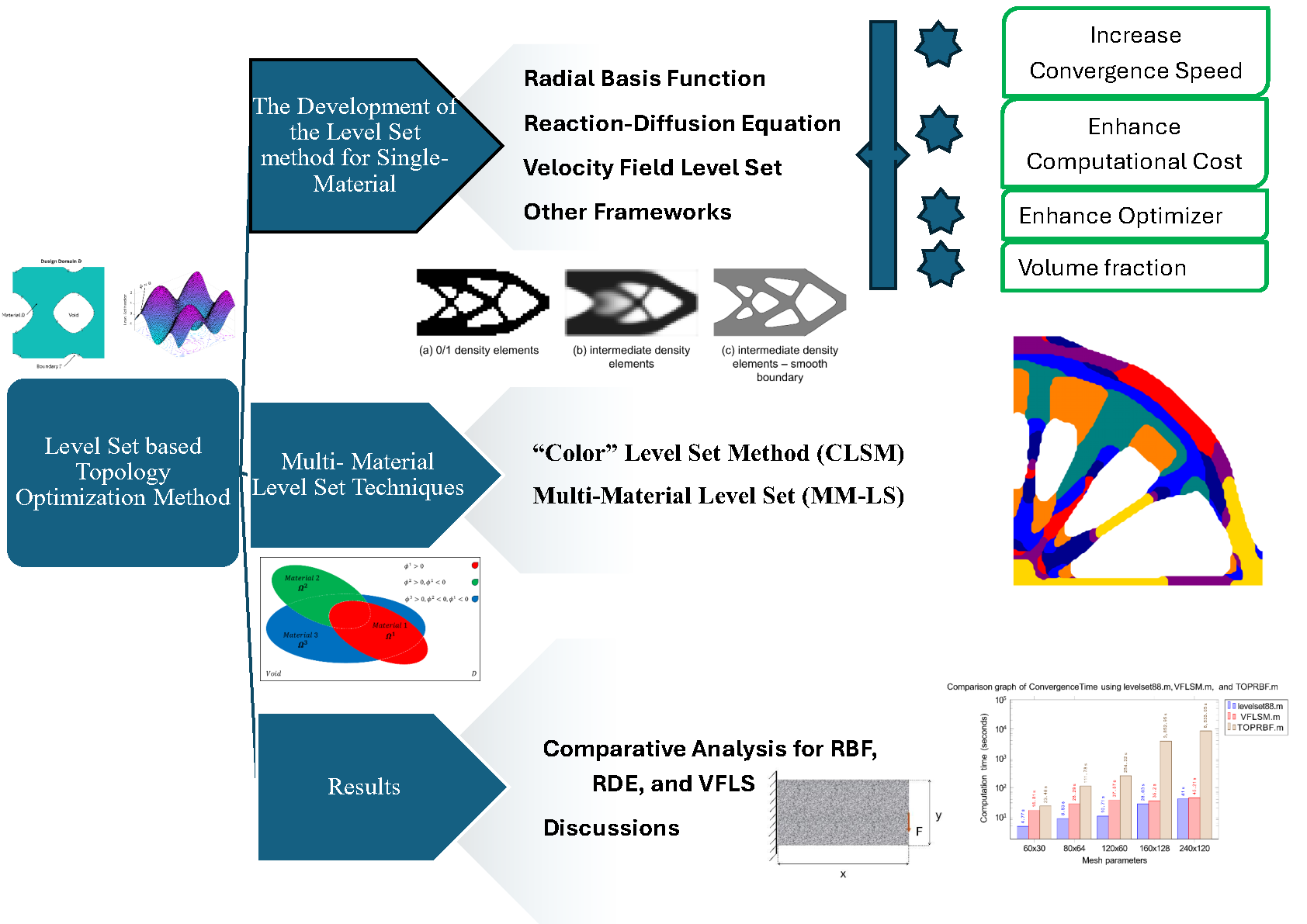
Figure 1. The review paper framework.
Van Dijk et al.’s (2013) research summarizes methods for implementing LSM models and discusses the advantages and disadvantages of different level set methods. In this study, different approaches to the level set method are presented separately to highlight the development process of each approach. Different from Van Dijk et al.’s (2013) research, this study focuses on improving methods in structural optimization, including reducing the number of convergence iterations, computer resources, computation time, volume fraction, and the objective function. Therefore, the advantages and disadvantages of the methods in this study are visually demonstrated in the results, along with the limitations encountered. This can then suggest directions for future research or areas for improvement.
During the review process, published studies with accompanying educational codes will be noted. These notes provide readers with options for experimenting with and learning about LSM. Finally, another new aspect of this review is the use of three corresponding educational codes for three typical approaches: Radial Basis Function, Reaction-Diffusion Equation, and Velocity Field Level Set method. These approaches will be directly compared on the same computing device (personal computer) for the cantilever beam problem. The results show that the Reaction-Diffusion Equation method offers a more balanced set of advantages for further optimization or development in complex optimization, such as multi-material optimization.
The following sections of this paper are presented in the following order. Figure 1 presents various analytical perspectives on the optimization of the level set structure, based on selected articles relevant to the goals of this paper, including radial basis functions, the reaction-diffusion equation, the velocity level set method, and other frameworks, as well as multi-materials. These sections also present open-source codes. The comparative analysis section discusses prominent methods, their comparisons, and discussions. Finally, last section gives the conclusions.
The Development of the Level Set Method for Single Material
Problem of Unified Theoretical Framework
In this study, papers using the level set method are selected based on criteria such as convergence speed, computation cost, optimizers that accelerate convergence or enable void creation, and volume fraction, to form a unified theoretical framework for the entire analysis. This approach distinguishes this review from others (Feng et al., 2018; Gibou et al., 2018; J. Liu et al., 2018) in its synthesis of studies, as it presents analyses based on results according to the four criteria mentioned above. These criteria were selected for the analysis for the following reasons:
Convergence speed is often one of the factors reflected in the results of topology optimization research. Although not explicitly stated, some studies use the number of convergence iterations to demonstrate that a new method is more optimal than a previous one . However, the total time required for convergence has not been analyzed as an important parameter, which must be related to the total number of iterations. There are two reasons that necessitate this correlation: firstly, optimization studies for the smoothness of the optimized shape or for multi-material may require up to 200, 300, 500, or even 1500 iterations (O. Sigmund, 2007; Sugimoto et al., 2024; F. Wang et al., 2011; Zhao & Zhang, 2021; R. Zheng et al., 2024) . Secondly, when comparisons are needed, the time per iteration is a better comparative metric than the number of iterations only, because a small number of iterations can result in a very long time.
Table 1. Visualization of the review purposes on the level set method for single material.
|
Purpose of the Level Set based Topology Optimization method review | |
|
Improvement of Convergence Speed | |
|
Enhance Computational Cost | |
|
Enhance Optimizer | |
|
Volume Fraction | |
One challenge in topology optimization research is the hardware requirements of computer configurations (Wegert et al., 2025; S. Xu et al., 2022; Yago et al., 2022) . This research focuses on studies that can work efficiently on personal computers, which are suitable for most new researchers. This efficiency not only achieves optimal performance on the current problem, but it also assesses the ability to develop complex structures, such as optimizing 3D structures or multi-material problems, while maintaining optimal performance on personal computers.
The presence of voids increases the complexity of the optimized geometry during topology optimization. In other words, creating many voids is considered optimal for the method. Some level set approaches, including conventional level set method (Wei & Paulino, 2020), find it difficult to create new voids, so optimizers such as volume integration schemes are needed to generate them in the initial step, thereby speeding up convergence (Wei et al., 2018; Wei & Paulino, 2020) .
The volume fraction is one of the final results of the optimization process. Most studies reported this value only as numerical values that converged, such as 0.5 or 0.45, without deeper discussion. Only a few studies show that this result depends quite heavily on intermediate elements and the Lagrangian augmentation method (Y. Cui et al., 2023), which is widely used in research. For single-material studies, the constrained volume is usually large, for example, 0.5, so the volume fraction result is usually very close to the constrained volume. However, when optimizing across multiple materials, each material has a very small volume, leading to a significant discrepancy between the constrained and optimized volumes. This summary will demonstrate this discrepancy in multi-material optimization studies, where authors also avoid providing these values.
From the optimization perspective, studies that focus on the level set method for single-material to improve convergence speed, reduce computational cost, enhance the optimizer, and improve volume fraction are considered. Each purpose is presented in Table 1, and the studies corresponding to each purpose are detailed below.
Radial Basis Function
The work of Wei et al. (2018) for Radial Basis Function (RBF) is chosen as the reference benchmark in this study. The first reason is that Wei et al. (2018) introduced 88 lines of MATLAB code for educational purposes. Second, this work used a volume integration scheme to increase optimization speed by starting with a lower volume fraction (see Figure 2).
Wei and Paulino (2020) improved the RBF method by using unstructured polygonal finite element models, enabling optimization of more complex shapes, higher accuracy, and clearer material-void boundaries without the need for additional smoothing methods. Wei and Paulino (2020) also replaced the Hamilton-Jacobi equation with a system of ordinary differential equations (ODE) to update the level set function. However, the results showed no significant improvement in convergence speed.
Figure 2. An example of the optimization process of the cantilever problem using mesh size. (a) the boundary conditions ; (b) initial holes distributed in volume integration scheme; and (c) optimized geometry.
Andrade and Santos (2022) used the Hilbertian extension to update the sensitivities along with the RBF method. In this method, a velocity field is created, reducing the dependence on the mesh of the previous method (which only used the natural normal velocity field). Andrade and Santos’s (2022) research also used the Ersatz material approach (Laurain, 2018) to achieve smoother density element values. Specifically, the Young's modulus of the voids is assigned a very small value (i.e., 1e-4) rather than 0, and the material's Young's modulus is set to approximately 1, creating a continuous cover zone around the boundary and resulting in a more seamless boundary. While this offers more advantages than the previous approach, using the Hilbertian extension increases computation costs.
In 2024, Sobczak and Sokół used RBFs and Hilbertian descent direction to approximate the level set function and performed their analysis using the Wolfram Mathematica code platform. The novel contribution of Sobczak and Sokół (2024) was the application of the analytical exponential formula in level set problems to reduce the number of iterations required for convergence. However, the study did not directly compare computation time with other studies due to differences in coding environments. In addition, this study focused on capturing the optimal shape, ignoring the presence of some free solid elements in the void domain.
In the same year, J. Zheng et al. (2024) published an improvement to the traditional RBF method that significantly improved computational performance. J. Zheng et al.’s (2024) method combined RBF with finite difference to create a meshless method based on local differentiation construction, namely RBF-FD-PLSM, thereby controlling the computational matrix.
Acceleration of Convergence (RBF Approach)
Table 2 summarizes the convergence speed of radial basis function optimization problems from some prior researches. These values were achieved when computer computing speeds were still relatively underdeveloped. Based on the convergence iteration count, it can be seen that with the same approach, although performed in 2006, S. Wang & Wang’s (2006) results are significantly better than Luo et al. (2009), as the problem converges at a low number of iterations. Furthermore, in terms of computation time, Luo et al.’s (2009) study required only 45 seconds/iteration at a finer mesh of 7200 elements, whereas S. Wang & Wang’s (2006) study required 287 seconds/iteration at a mesh of 3200 elements. Therefore, there is reason to believe that Luo et al.’s (2009) study improves on S. Wang & Wang’s (2006) with respect to the influence of computation time/iteration.
|
Research |
Mesh parameter (Size parameter) |
Calculation Time (seconds) |
Iteration |
Computational resources |
|
|
543.8 |
34 |
CPU Intel Pentium IV processor of 3.4 GHz | |
|
|
4,595 |
59 | ||
|
|
9,761 |
34 | ||
|
|
- |
142 |
CPU processor of 3.06 GHz with 2 GB RAM | |
|
|
- |
153 | ||
|
|
16,785 |
373 |
- |
Meanwhile, in recent studies, as computation speed has improved across both hardware and programming methods, convergence speed should be measured as the number of convergent iterations and the total computation time and reported as the computation time per iteration.
|
Research |
Mesh parameter (Size parameter) |
Calculation Time (seconds) |
Iteration |
Volume fraction
|
Computational resources |
|
Radial Basis Function | |||||
|
|
- |
100 |
0.4996 |
- | |
|
|
- |
102 |
0.5001 | ||
|
1000 |
- |
100 |
0.5 |
- | |
|
|
62.4 |
48 |
0.5 |
CPU Intel Core i7-7500U, 2.7 GHz, with 16 GB of RAM | |
|
|
71.5 |
55 | |||
|
|
79.3 |
61 | |||
|
|
- |
50 |
- |
- | |
|
| |||||
|
| |||||
|
|
11.64 |
97 |
0.5 |
Intel i5-1135G7 CPU | |
|
Serpentine domain |
29.03 |
175 | |||
|
Hook domain |
28.44 |
165 | |||
Convergence speed is one of the values that reflects the optimality of a method. The faster the convergence speed, the more efficient the method. Fast convergence speed must be accompanied by accurate objective function values within the constraints. When the result satisfies the objective function, the convergence speed should be measured by both the number of convergence iterations and the convergence time. As shown in Table 3, the data collection computation cost to complete the optimization in radial basis function approach should be considered.
Wei et al. (2018) and Wei and Paulino (2020) both achieved similar convergence speeds at around 100 iterations; however, the computation time for their methods was not specified, making direct efficiency comparisons difficult.
In contrast, Andrade and Santos’s (2022) research significantly reduced the number of iterations required for convergence, with only 48 and 61 iterations for and mesh sizes, respectively. Moreover, Andrade and Santos (2022) reported iteration time of 1.3 seconds contributed to a notably shortened optimal time.
J. Zheng et al.’s (2024) study showed significantly faster convergence, requiring only about 0.13 seconds/iteration when calculating irregular design domains (including Serpentine and Hook domains). However, when comparing only the number of iterations required for convergence, J. Zheng et al.’s (2024) study required the most, more than Wei et al.’s (2018) study, and nearly three times as many as in Andrade and Santos’s (2022) study.
Computational Cost (RBF Approach)
In Andrade and Santos’s (2022) work, the numerical examples were run on a CPU Intel Core i7-7500U, 2.7 GHz, with 16 GB of RAM. J. Zheng et al. (2024) MATLAB code was run on an Intel i5-1135G7 CPU for the problems, demonstrating a significant reduction in computation time in a single iteration, with up to 90% faster in time per iteration compare to Andrade and Santos’s (2022) work for the minimum compliance problem.
From these two studies, significant advancements in method optimization and coding have been observed, enabling personal computer configurations to produce results much faster without requiring a high-performance computer for less complex problems.
Improvement of the Optimizer (RBF Approach)
Optimization Initial Design
The advantage of creating holes in the initial computational domain (Dunning & Alicia Kim, 2013) is to help reduce the initial volume constraint value at the beginning of the optimization, while still maintaining the stability and reliability of the optimized structure. Reducing the value of this volume constraint is also used to optimize computational cost, such as the total number of iterations and the total convergence time, but in practice, it can yield different results across methods under the same computational conditions. In addition, the stability of the geometry after optimization, also depends on the number, size, and symmetry (see Figure 2 (b)) of the initial holes. Therefore, in most methods that use initial holes, many small holes are placed symmetrically and evenly in the computational domain. Many studies have introduced methods for creating holes (Allaire et al., 2004b; Belytschko et al., 2003; Burger et al., 2004; Gomes & Suleman, 2006; He et al., 2007; Sethian & Wiegmann, 2000; S. Wang & Wang, 2006; Yamada et al., 2010) in the early stages, but Dunning & Alicia Kim’s (2013) research helps establish the connection between boundary propagation and the creation of new holes, enabling smooth convergence to optimal solutions.
Note that the initial holes in the volume integration scheme are not non-design holes (Andreassen et al., 2011; O. Sigmund, 2001) , and will continue to be transformed into material or voids in subsequent iterations (Han et al., 2021). Although the initial holes in the volume integration scheme may continue to transform, their appearance affects the result, for example, making the optimized geometry asymmetrical when the initial holes are too large, or placed asymmetrically, or when the number of holes is too small (1 to 3 holes).
The optimization process begins by first creating holes in the computational domain (Andrade & Santos, 2022; Wei et al., 2018; Wei & Paulino, 2020; J. Zheng et al., 2024) . After initializing the holes at this initial stage, the volume is reduced, and the method then predicts the random distribution of holes during optimization.
Optimization Strategy
Andrade and Santos (2022) used the Hilbertian extension to update sensitivities without reinitialization and, combined with decoupling the finite element mesh for the discretized structural design domain from the parameterization mesh, enhanced both optimization efficiency and accuracy.
J. Zheng et al. (2024) introduced a new approach that radial basis function generated finite difference (RBF-RD) was used to develop a new parameterized level set method (PLSM). The new RBF-FD-PLSM can work for both regular and complex design domain, with rectangular and polygonal elements, respectively.
Volume Fraction (RBF Approach)
The augmented Lagrange method was used to control volume constraints (Andrade & Santos, 2022; Wei et al., 2018; Wei & Paulino, 2020; J. Zheng et al., 2024) . In Wei et al.’s (2018), Wei & Paulino’s (2020), Andrade & Santos (2022), and J. Zheng et al (2024) studies, the volume fraction at convergence approximated the constrained volume ratio.
Remark on Existing RBF Methods
In the studies analyzed, studies of J. Zheng et al. (2024) and Andrade and Santos (2022) fully demonstrate the values of interest in this research framework. J. Zheng et al. (2024) used PYTHON, which may give difficulties for new researchers due to the lack of necessary libraries (e.g., FEniCS, DOLFIN) that require installation via technically demanding efforts or execution on colab.research.google. J. Zheng et al. (2024) had the lowest convergence time but yields the largest number of iterations and does not yet achieve optimal results for the finer-mesh parameter. The remaining studies lacked many of the necessary results for this research; however, Wei et al.’s (2018) study provided a concise code snippet that applies the sparse function (Andreassen et al., 2011) to reduce the computational matrix, which could be used for the development of multi-material optimization.
Reaction-diffusion Equation
Otomori et al. (2015) further developed the level set method incorporating a fictitious interface energy from Yamada et al. (2010), and used the reaction-diffusion equation to introduce and provide MATLAB code for educational purposes. Similar to Wei et al.’s (2018) research on the RBF approach, Otomori et al.’s (2015) research is also selected as the benchmark for comparison with the RDE approach.
In Otomori et al.’s (2015) research, the exact Heaviside function (Van Dijk et al., 2012) was chosen to project the values of the level set function onto the elements of the computational domain as 1 (material) or 0 (void). The level set function is updated using the reaction-diffusion equation instead of the Hamilton-Jacobi equation, providing the ability to generate complex voids without using a volume integration scheme.
To improve the efficiency, robustness, and stability of the optimization process, Seong et al. (2018) used the modified conjugate gradient method (CGM) in combination with the RDE technique. In this approach, the modified conjugate gradient method (CGM) helps reduce the number of intermediate density elements. The results showed that the volume fraction value approached the constraint volume, but the convergence rate did not improve significantly.
One of the four objectives of this review is the volume fraction (Table 1). The volume fraction is the distribution of material volume achieved during optimization, based on the volume constraint requirements. Therefore, the volume fraction must converge to the constrained volume. However, the number of intermediate density elements can affect this volume fraction (Y. Cui et al., 2023); specifically, as the number of intermediate density elements increases, the volume fraction value increases. Additionally, the augmented Lagrangian equation can also cause differences in this volume fraction (Y. Cui et al., 2023).
The first approach to limit the number of intermediate elements is to use the Heaviside function, as studied by Otomori et al.’s (2015). However, using the Heaviside function also has drawbacks, such as a zigzag shape of the material boundary when the mesh is sparse, or many iterations are required. Therefore, a second way to achieve a volume fraction with small error is to optimize the finite element mesh to reduce the number of intermediate density elements. Zhuang et al. (2021) used body-fitted mesh with triangular or tetrahedral meshes for more accurate results and smoother material boundaries. Wang et al. (2022) introduced a new method, called RDBLS, that combined B-spline functions with RDE, significantly enhancing optimization performance and efficiency across even complex computational domains.
Recently, the third method to improve the accuracy of volume fraction convergence was to replace the augmented Lagrangian equation with the exact constrained volume method introduced by Y. Cui et al. (2023). Y. Cui et al. (2023) introduced new approaches to accurately determine the exact Lagrangian multiplier for volume constraint control, which helped to achieve the exact constrained volume result for the RDE. In the density approach, the constraint volume is kept constant from the first computation iteration, along with control of intermediate density elements, to achieve superior accuracy in the converged volume value. Along with improving performance, the robustness of the optimized structures is also being further studied by Oka and Yamada (2023), specifically for nonlinear diffusion equations.
Acceleration of Convergence (RDE Approach)
As shown in Table 4, the data collection computation cost to complete the optimization in reaction-diffusion equation approaches should be considered.
As mentioned, Otomori et al.’s (2015) study was used for comparison with other studies that used the same reaction-diffusion equation approach. Although Otomori did not present the results in the original study, Zhuang et al. (2021) re-ran Otomori's code in his study for comparison. In the comparison presented, the RDE method with the non-body fitted mesh required significantly fewer convergence iterations than the fixed rectangular-mesh RDE method and the soft-killed BESO method, by 71.15% and 59.46%, respectively, for the cantilever problem. These results demonstrate that the mesh significantly affects the problem's convergence speed. However, the minimum compliance function results did not differ significantly, by less than 5%. Furthermore, the convergence time results were not discussed in this paper, thereby failing to fully demonstrate the optimization of computation time achieved by this new RDLS method.
The results of Wang et al. (2022) indicated that for a 2D cantilever beam, the RDBLS method required 18 iterations, completing the process in 101.1 seconds (5.617 seconds/iteration). In comparison, the Otomori's code required 104 iterations and took 146.7 seconds. For the MBB beam, the RDBLS method required 18 iterations and completed in 94 seconds, while the Otomori's code required 96 iterations and took 140.5 seconds. The results showed that with the new method, the number of iterations needed to converge was reduced by 82%, and the total time was reduced by 31% compared with the Otomori et al.’s (2015) results in the case of the cantilever beam. In 3D optimization, 50 iterations were sufficient to achieve convergence for a structure with approximately one million elements.
The convergence values of Oka and Yamada (2023), ranging from 64 to 414 iterations for optimization problems, are dependent on the value of , an appropriate number of eigenfrequencies from the lowest eigenmode (). Y. Cui et al. (2023) needs 101 iterations to converge the problem, and requires 2.367 seconds/iteration.
|
Research |
Mesh parameter (Size parameter) |
Calculation Time (seconds) |
Iteration |
Volume fraction
|
Computational resources |
|
Reaction-Diffusion Equation | |||||
|
|
- |
- |
- |
- | |
|
| |||||
|
| |||||
|
|
- |
100 |
0.5 |
- | |
|
|
- |
100 |
0.2 | ||
|
|
- |
30 |
0.501 |
- | |
|
|
- |
36 |
0.500 | ||
|
|
- |
37 |
0.2 | ||
|
|
- |
24 |
0.3 | ||
|
|
101.1 |
18 |
0.3 |
Intel(R) Core(TM) i5-8250U CPU with 256 GB of RAM | |
|
|
94 |
18 |
0.3 | ||
|
|
- |
50 |
0.3 | ||
|
(ratio) |
- |
64 414 |
- |
- | |
|
16512 |
239.1 |
101 |
0.4 |
- | |
Computational Cost (RDE Approach)
The computational domain size was , which was computed using an Intel(R) Core(TM) i5-8250U CPU with 256 GB of RAM in Wang et al.’s (2022) research.
Improvement of the Optimizer (RDE Approach)
Seong et al. (2018) replaced the steepest descent method with a modified conjugate gradient method, thereby improving convergence. Zhuang et al. (2021) used a body-fitted mesh and updated the Lagrange multiplier using a bisection method to increase accuracy and improve convergence. Y. Cui et al. (2023) replaced the augmented Lagrangian method with the exact volume-constraint method to achieve the lowest volume fraction error.
Volume Fraction (RDE Approach)
In Seong et al.’s (2018) work, the penalty parameter increases the influence of volume constraints when used with the conjugate gradient method. Specifically, when the conjugate gradient exceeds the initial gradient, the penalty parameter is increased to accelerate convergence of the constraint. However, before convergence, the volume fraction curve also experiences large, continuous fluctuations.
Zhuang et al. (2021) used an RDE with a body-fitted mesh to achieve high accuracy in the volume fraction results. Compared to a fixed rectangular mesh for the cantilever beam problem, although both used the augmented Lagrangian method to control the volume fraction, the volume fraction results for the fixed rectangular mesh and body-fitted mesh problems were 0.5035 and 0.501, respectively. In the MBB problem, the volume fraction results obtained for the fixed and non-body-fitted meshes were 0.5048 and 0.500, respectively.
Wang et al. (2022) continued to use the bi-sectional and body-fitted mesh method, resulting in volume fractions in the 2D problem with an error of less than 0.01. Y. Cui et al. (2023) used the exact volume-constraint method instead of used the augmented Lagrangian to control the volume constraint, and the results showed that this method not only achieved a volume fraction with an error of less than 0.001, but also prevented large fluctuations in the volume fraction graph.
Remark on Existing RDE Methods
In the studies analyzed, only Otomori et al.’s (2015) study lacks all the values of interest in this research framework. Nevertheless, other results in Otomori et al.’s (2015) study demonstrated the potential for further development of multi-material optimization, as it provides concise code and uses sparse functions (Andreassen et al., 2011) to increase computation speed and reduce computation cost by reducing the matrix size. The remaining studies demonstrate the stability and effectiveness of the RDE approach. The difference between these methods is that studies Zhuang et al. (2021) and Wang et al. (2022) modify the mesh in the finite element model, whereas Y. Cui et al. (2023) used the exact volume-constraint method rather than the augmented Lagrangian method.
Velocity Field Level Set and Other Computational Frameworks
Returning to the technique of updating the level set function using the Hamilton-Jacobi equation, Wang and Kang (2018) introduced a new approach that uses the velocity field to evolve the design boundaries, called the Velocity Field Level Set. Wang and Kang’s (2021) further developed this technique, using Svanberg’s (1987) Method of Moving Asymptotes (MMA) optimizer to accelerate convergence and produce a smoother optimal geometry. Wang and Kang’s (2021) also provided MATLAB code for this approach, for educational purposes, so this review uses Wang and Kang’s (2021) research as a reference for comparison. In the following studies, the authors continue to improve stability and apply other constraints, such as stress constraints by Cheng et al. (2024) and the irregular level set grid by (Jia et al., 2026). With the body-fitted mesh based approach already achieving optimal results, Zhuang et al. (2024) further developed a new method, the estimated Gradient Field (GFLS). This new method, combined with the body-fitted mesh, significantly increased convergence speed while maintaining very high accuracy in the volume fraction. In addition to studies completed with MATLAB, other programming platforms were applied to level-set-based topology optimization research. Laurain (2018) developed a Python-based system using the FEniCS solver to calculate compliance minimization in structural optimization. Chung et al. (2019) used NASA’s OpenMDAO framework to demonstrate the capabilities of its computational tools for developing topology-optimized structures. Chung et al.’s (2019) research was completed for both LSM and SIMP.
In 2023, Jauregui et al. had developed open-source software for a level set optimization approach, called ParaLeSTO. The aim was to modularize topology optimization methods, thereby increasing reusability and enhancing interactivity for the academic community by creating metadata. In addition to using the FEniCS analysis platform, ParaLeSTO software also includes PETSc and COMSOL analysis. Following the use of open-source computing platforms, specifically the Portable Extensible Toolkit for Scientific Computing (PETSc), Wegert et al. (2025) introduced an extensible framework for level set optimization called GridapTopOpt, implemented in Julia. Wang and Kang’s studies in 2018 and 2021 used the same VFLS approach, yielding similar computational speed results for both 2D and 3D problems.
In Laurain’s 2018 work, the cantilever beam numerical example benchmark with the mesh size required 60 iterations to convergence, and the time result was 4.933 seconds/iteration. When the mesh size was increased to , the computation time was 13.171 seconds/iteration for 82 iterations. The highest calculation time was 33.429 seconds/iteration in mesh size.
Acceleration of Convergence (VFLS and Other Computational Frameworks)
|
Research |
Mesh parameter (Size parameter) |
Calculation Time (seconds) |
Iteration |
Volume fraction
|
Computational resources | |
|
Velocity Field Level Set | ||||||
|
|
- |
88 |
0.5 |
- | ||
|
|
- |
46 |
0.5 | |||
|
|
- |
158 |
0.3 | |||
|
|
- |
59 |
0.5 |
- | ||
|
|
- |
68 |
0.45 | |||
|
|
- |
164 |
0.1496 | |||
|
Other Computational Frameworks | ||||||
|
|
- |
98 |
0.5 |
- | ||
|
|
- |
73 |
0.4 | |||
|
|
296 |
60 |
- |
CPU Intel Core2 Q9400, 2.66 GHz, with 3.8 GB of RAM | ||
|
|
1,080 |
82 |
- | |||
|
|
8,257 |
247 |
- | |||
|
|
- |
- |
0.4 |
- | ||
|
|
900 |
167 |
0.4 |
144 Intel Xeon Platinum 8274 Processors with 4GB per core on the Gadi NCI Australian supercomputer | ||
|
|
2,280 |
108 |
0.4 | |||
|
|
- |
121 |
0.4 | |||
|
|
- |
24 |
0.4999 |
CPU Intel Core i7-12700H, 2.30 GHz | ||
|
|
- |
22 |
0.5001 | |||
|
|
- |
21 |
0.4002 | |||
|
7859 |
89.8 |
24 |
- | |||
The most impressive results came from Zhuang et al.’s (2024) research, which, using a standard computer configuration, achieved a speed of 3.742 seconds/iteration for the 2D problem, requiring only 24 iterations to achieve optimal results. In another study Wegert et al. (2025), a supercomputer was used to solve the 3D problem with a large mesh (3,375,000 elements), yielding a per-iteration computation time of 5.389 seconds.
Computational Cost (VFLS and Other Computational Frameworks)
All numerical tests of Laurain (2018) were run on a CPU Intel Core2 Q9400, 2.66 GHz, with 3.8 GB of RAM. To solve PDEs and adapt the code for multiphysics problems, this study demonstrated the strength and efficiency of FEniCS, making it a reliable and cost-effective tool for structural topology optimization that utilizes the level set technique.
Zhuang et al.’s (2024) research used a computer with a basic configuration: a 2.3 GHz CPU Intel Core i7 12700H. Using the novel GFLS method, Zhuang's results achieved better optimization than the BESO (Zhuang et al., 2023), BFLS-UPWIND (Allaire et al., 2014), and HJLS (Challis, 2010) methods, all calculated on the same configuration, achieving the smallest objective function value, a low number of iterations to convergence, and optimal shape quality. The GFLS method's compilation cost was 43.39% and 8.39% lower than those of the BFLS-UPWIND and HJLS methods, respectively.
Wegert et al.’s (2025) study was the only one to use a supercomputer, demonstrating significant efficiency in computing complex (3D) and fine-mesh problems (over 3 million elements), requiring only 167 iterations in approximately 900 seconds.
Improvement of the Optimizer (VFLS and Other Computational Frameworks)
The VFLS method used the implicit function and Hamilton-Jacobi equation, constructed with velocity field to enhance the efficiency of multiple constraints. This approach still uses the Hamilton-Jacobi equations, similar to the RBF approach, then using an MMA solver as optimizer. In the following studies, the authors continue to improve stability and apply other constraints, such as stress constraints by Cheng et al. (2024).
Volume fraction (VFLS and Other Computational Frameworks)
All the studies above used the augmented Lagrangian technique to control volume fractions. The results were all very accurate and consistent with volume constraints, with Zhuang et al.’s (2024) volume fractions achieving particularly high accuracy. Zhuang et al. (2024) had once again succeeded with the body-fitted mesh, combined with the Gradient Field.
Remark on Existing VFLS Methods
The VFLS method is being developed by a group of authors, and there is little research in the community. This has the advantage of leaving a research gap for further studies, but the disadvantage is that the development area is narrow and may conflict with the main author group. A second weakness of the VFLS method is that, although the published code is short and very suitable for research and development, the authors use Svanberg’s (1987) MMA function; therefore, the actual code is much longer than described, making it less attractive for customization.
Multi-material Level Set Techniques
The Importance of Multi-material Optimization
The advantages of topology optimization methods have been described and demonstrated in studies of single materials. To apply these advantages to practice, problems with multi-materials are necessary. With a large number of outstanding studies, multi-material optimization using the SIMP technique has achieved significant results. Using optimization for multi-materials can achieve better strength-to-weight ratios, optimize costs when combining different materials for the same structure (Bohrer & Kim, 2021; Doan et al., 2020) , or be applied to layered-material structures (Tajs-Zielińska & Bochenek, 2021). In practical applications, such as in the automotive field, Shah et al. (2023) developed a prototype design for a lightweight electric all-terrain vehicle (eATV) chassis by combining titanium, aluminum, and carbon fiber sheet molding compound. In the aerospace field, critical aircraft structures such as the aircraft pylon, engine bracket, and front fuselage have also been studied for topology optimization applications (Zhu et al., 2016b).
In optimization involving graded porous materials, studies by Bruggi et al., (2022), Wu et al. (2018), and Schmidt et al. (2019) show that the distributions of the solid phase of the material, a graded porous phase, and a void are a form of multi-material optimization, where the graded porous phase value lies between 0 (void) and 1 (solid phase). In practice, graded porous materials are used for bone screws or bone-like structures (Wu et al., 2018; Zhao & Zhang, 2021) to improve the mechanical and biological properties of porous osseointegrated screws (Yang et al., 2024).
The development of level set methods for multi-material optimization emerged nearly a decade after SIMP, in 2004 (M. Y. Wang & Wang, 2004) rather than 1997 (J. Liu et al., 2018; 0 Sigmund & Torquato, 1997; R. Zheng et al., 2024) , respectively. Nevertheless, research and applications of level set methods have made important progress, particularly MM-LS techniques, which offer high customization and the potential to develop new approaches.
The section on multi-materials will discuss methods for distributing different material types within the design domain by controlling level set functions. There are many different ways to control level set functions, and this study will classify and analyze these control methods.
“Color” Level Set Model Method (CLSM)
As shown in Figure 3, a method called CLSM (M. Y. Wang & Wang, 2004), defines up to four phases for the distribution of two materials defined by two level set functions. The intersection of 2 materials is defined to exist when and , material 1 appears when and , material 2 appears when and , and voids appear when both and negative. Then, material 1 is distributed in the intersection area. Therefore, for each of material, the number of phases is .
The fact that the number of phases is , where is the number of materials to be optimized in the computational domain, leads to a significant increase in the number of phases as the number of materials increases. This makes it difficult to control the phases, or adds pressure on the computational equation.
Figure 3. The ‘Color’ Level set for multi-material strategies: M = 2 materials, .
Due to the disadvantage of increasing the number of materials to be optimized, the CLS method has not been widely adopted, and most studies stop at 4 phases, including voids (corresponding to 2 level set functions). Nevertheless, some studies have taken advantage of the CLS method's such as ability to generate 3 material phases from 2 level set functions, as well as its smooth phase transitions at boundaries and prevent the material overlap, such as Zhou et al. (2022) researched on multiphase auxetic metamaterials, Ghasemi et al. (2018) researched on flexoelectric composites, and P. Liu et al. (2016) used the union phase to define the bonding interface.
Multi-material Level Set (MM-LS) Method
To overcome the shortcomings of the CLSM method, Wang et al. (2015) introduced a completely new approach in which the total number of materials and void in the computational domain to be optimized equals the total number of phases, M+1, where M is the total number of materials. Thus, the number of phases for the material (excluding voids) is also equal to the number of level set functions. This approach makes controlling the level set functions easier and makes increasing the number of materials to be optimized more feasible. Furthermore, the fact that the number of phases for the material (excluding voids) equals the number of level set equations also facilitates the development of new methods based on MM-LS, as analyzed below.
First and original, the expression for cases with up to three materials in Wang et al.’s (2015) research is represented in Figure 4. The is used to define the solid or void phase; therefore, in any area where , the void has appeared. The is used to present material 2 in the solid phase when . When , the rest of the solid phase is defined by material 1. Material 3 appears in the material 2 zone when . In case , the material 2 zone is not replaced.
Figure 4. Original MM-LS scheme for 3-material (4 phases).
According to Y. Wang et al. (2015), material occurrence was governed by level set functions. The main difference from the CLSM method was that a single level-set function () controlled the occurrence of all materials. Under the conditions for material occurrence, this level set function should always be positive; when it is negative, voids will appear. For consistency with other methods, Table 6 presents the conditions applied for three materials: code A indicates material occurrence, while code B indicates voids.
Table 2. Summary table of convergence rates of several older studies using the Radial Basis Function based level set method.
Table 3. Computational cost of Radial Basis Function based level set method.
Table 4. Computational cost of Reaction-Diffusion Equation based level set method.
Table 5. Computational cost of the Velocity Field Level Set method.
Table 6. The condition of the materials and the void phases in 3-material case.
|
Condition |
Phases |
Functions | |
|
A-3 |
Material |
| |
|
A-2 |
Material |
| |
|
A-1 |
Material |
| |
|
A-0 |
Material |
| |
|
B-1 |
Void |
| |
|
B-2 |
Void |
| |
|
B-3 |
Void |
| |
|
B-4 |
Void |
| |
|
where ; is the number of materials | |||
Material 1, material 2, and material 3 denote materials of increasing stiffness: softest, medium, and hardest, respectively. Figure 5 shows the order and appearance conditions of these materials in Y. Wang et al.’s (2015) study, where the hardest material (material 3) appeared first.
Figure 5. Diagram of the possible material distribution under the condition in Wang et al.’s (2015) research.
Nguyen-Tran et al.’s (2025) research applies the exact volume constraint (Y. Cui et al., 2023) with MM-LS. In the 3-material problem, material 3 appears under condition , and material 2 appears under condition . Material 1 occurs for all values of , while the void state occurs for all combinations of and , but only when is less than 0 . The study by Nguyen-Tran et al. (2025) used the same material reconstruction conditions as in Y. Wang et al.’s (2015) original study. The difference is that the softest material (material 1) appeared first under the same A-0 and A-1 conditions, as shown in Figure 6.
Figure 6. Diagram of the possible material distribution under the condition in Nguyen-Tran et al. (2025) research.
Next, M. Cui et al. (2016) applied the RDE technique to the improved MM-LS method, using all level set functions simultaneously to control the occurrence of each material. In M. Cui et al.’s (2016) study, the application of level set functions for material reconstruction was modified. Unlike Wang's original study, in which all conditions in code A were used to reconstruct the materials, M. Cui et al.’s (2016) study adjusted the application to use only one condition for each material, as shown in Figure 7.
In this case, the condition A-2 in code A is also presented as void (see Figure 8). However, since condition A-2 still has , a material currently under condition A-2 can be transformed into conditions A-1 and A-3 if any level set function, or , changes sign. This phase shift is weak, but it is still possible if the conditions defined by the sign of the level set function are met. The advantage of M. Cui et al.’s (2016) method is that the material reconstruction rate for each material is mathematically identical, making it suitable for more than three materials when each is defined by only one condition.
Figure 7. Modified MM-LS scheme for 3-material (4 phases) by M. Cui et al. (2016).
However, the initial appearance of the weakest material can make it difficult to replace voids later in practice. To explain this disadvantage in detail, initially, the softest material appears throughout the entire domain. When hard materials replace the load-bearing areas, the softer materials must redistribute to support the structure. Nevertheless, these areas may already have been replaced by voids (condition code B). This makes it difficult for the softest material to replace them, because it increases compliance. There is evidence in Cui's results that the softest material appears as small dots around the harder material.
Figure 8. Diagram of the possible material distribution under the condition in M. Cui et al. (2016).
The approach in Wang et al.’s (2015) and Nguyen-Tran et al.’s (2025) method showed that all conditions with are used to determine the material, and that there is always a preference for a material with more conditions to appear, with Wang et al. (2015) prioritizing the hardest material, while Nguyen-Tran et al. (2025) prioritizing the softest materials. This selection can lead to over prioritization when increasing the number of materials to be optimized, and also create differences in the allocation of conditions for material reconstruction. M. Cui et al.’s (2016) method can adjust a material's condition to address this problem. However, improvements are still needed in the order of material appearance and in the systematic selection of conditions.
Figure 9. Modified MM-LS scheme for 3-material (4 phases) by Sha et al. (2021).
Using an alternating active-phase formulation and a difference-set-based multi-material level set (DS-MMLS) design, Sha et al. (2021) presented a revolutionary multi-material level set topology optimization technique. Sha et al. (2021) developed a new approach by using the MM-LS method; however, by applying the alternating active-phase methodology, the challenge of multi-material topology optimization can be transformed into a succession of binary-phase sub-problems (Sha et al., 2021). The sub-problems help reduce the number of variables and the volume constraints (Sha et al., 2021). First, material 1 will appear in the design domain where . Next, material 2 will appear in the region where , it must not overlap with the region where material 1 already exists. Then, according to the above principle, material 3 appears when , it must not overlap with the region of material 1 and material 2 before (see Figure 9).
Although Liu and Ma (2018) and Sha et al. (2021) also used the MM-LS method, their approaches shared some similarities with the CLSM method in defining the intersection region. Specifically, to optimize the level set using component-length-scale control on multi-material structures, Liu and Ma (2018) directly defined each level set function to represent each material phase, as shown in Figure 10, thereby freeing the dependent length-scale control. However, Liu and Ma’s (2018) research is limited to two materials, with materials 1 and 2 corresponding to level set functions 1 and 2, respectively, when they are positive. The intersection region between the two materials is defined as the intersection of two positive level set functions, assigned a stiffness value equal to 0.5 times the stiffness value of the softest material.
Figure 10. Modified MM-LS scheme for 2-material (3 phases) by Liu and Ma (2018).
Recent studies on multi-material level-set-based topology optimization (MM-LS) show that the method has been widely adopted and is developing rapidly. Only Sha and Nguyen's study optimized more than 3 materials, specifically 5. Other studies, especially Kumar and Rakshit (2025), although introduced in the methods section as optimizing for up to 3 materials, reported results that optimized only for 2 materials (see Appendix B).
The common point of these methods is that they all use the exact Heaviside function to determine the elastic stiffness for the materials, where when the conditions are met, the exact Heaviside function will set the corresponding level set values to 0 (void) and 1 (material), and assign them to the elastic stiffness values through equations (2) to (7).
Some Other Methods
Not limited to multi-material optimization for structures, the MM-LS method is also applied to other fields such as heat transfer problem (Shen & Feng, 2018; X. Xu et al., 2022, 2023) , electromagnetic problem (Tian et al., 2022), and coated structures with multiple infill materials (Bai & Zuo, 2022). This demonstrates the wide range of applications of the MM-LS method across multiple fields. In these studies, the MM-LS method is applied using approaches similar to those used in minimum compliance optimization. Although the MM-LS method has been applied in many studies, new methods have been introduced to supplement level set optimization. Several methods differ significantly from CLSM or MM-LS, such as Noda et al.’s (2022) extended level set (X-LS) method and Sugimoto et al.’s (2024) multi-phase-field multi-material topology optimization model.
The X-LS method treats voids as a material type, and a level set function defines a pair of materials. When this level set function is zero, it represents the boundary between the two materials. Because of this approach, the X-LS method for optimizing a problem with phases requires level set functions. For example, in a single-material optimization problem, with phases, the number of level set functions required is ; in a 3-material optimization problem (2 material phases + 1 void phase), with phases, the number of level set functions required is . It can be seen that with the X-LS method, increasing the number of materials requires more level set functions to control each material type than with the CLSM method. However, each function is precisely defined to manage a pair of materials within the total number of materials to be optimized, ensuring the problem remains feasible with the required number of materials. The X-LS method has demonstrated optimal efficiency for up to 9 materials (8 material phases and 1 void phase), showing its applicability.
As for Sugimoto et al.’s (2024) multi-phase-field multi-material topology optimization model, voids are treated as a material type, and each phase is defined by a level-set function, called a phase-field (PF). Sugimoto et al.’s (2024) method requires one additional level set function than the MM-LS method and has also proven effective, achieving optimal results for up to 6 materials (5 material phases and 1 void phase).
The Limitations of the Previous MM-LS and Future Works
The disadvantages are most evident when optimizing for multiple materials. First, the results do not show the total time to complete the iterations (except Kumar and Rakshit (2025)), so it is not possible to determine which approach is faster. The number of iterations varies across studies, depending on the author's purpose. Therefore, if the computation time per iteration were available, a comparison of convergence speeds between methods would be more appropriate.
The second concern is the volume fraction. Regarding volume fractions, materials within the multi-material computational domain often have low volume constraints, leading to larger discrepancies in volume fraction results when combined with intermediate elements and the augmented Lagrangian method. Specifically, previous studies did not provide precise results for the volume achieved after optimization; the results were only shown graphically (approximately). In particular, there were cases where the volume did not converge to the given constraint, such as Sha et al.’s (2021) study, which yielded a volume of approximately 0.28, while the constraint volume was 0.2. Similarly, in Kumar and Rakshit’s (2025) study, neither volume result converged to 0.25 as the constraint volume. Currently, only Nguyen-Tran et al. (2025) used the exact volume constraint to address this issue.
Analysis of the aforementioned multi-material optimization studies reveals that the results proposed in these previous studies have not been fully demonstrated by the previous authors, or may even be omitted or misjudged (Kumar & Rakshit, 2025b; Sha et al., 2021) . This creates a suitable research gap, where one or more new approaches are needed that fully represent computation speed (time per iteration), computational cost (to support the popular application of the method), and volume fraction (convergence criteria).
From these observations, it is clear that, in future research, the application of the MM-LS method in multi-material optimization still presents significant research gaps. First, the MM-LS method should be improved to use a single material per condition, and verified with more than three materials, as M. Cui et al.’s (2016) study failed to do. Next, the volume fraction value (accurate) should be improved compared to the constraint volume while still applying the Lagrangian augmentation method. Finally, the computation time value could be considered for presentation to develop the first comprehensive comparative study.
Results
Comparative Analysis for Single Material Approaches
From the summary Tables 3 to 5 above, studies provide relatively complete results for the number of loops, but the total time required to complete them is not fully published. When comparing the time required to execute one loop, the results show that the study of Andrade & Santos (2022); J. Zheng et al. (2024) - RBF; C. Wang et al. (2022) – RDE; and Zhuang et al. (2024) are the most optimal in iteration number and convergence time. Note that the device's computing power affects the computation time per iteration, but, interestingly, the results of these research show that the personal computer can be used to achieve the optimal results.
The Reaction-Diffusion Equation (RDE) (Otomori et al., 2015), Velocity Field Level set (VFLS) (Y. Wang & Kang, 2021), and Radial Basis Function (RBF) (Wei et al., 2018) methods all provide useful, open research code and are all executable on personal computers, making them more accessible to a wider range of researchers. However, the studies selected as references for each approach do not fully demonstrate the values that this review aims to achieve. Furthermore, the reason for selecting these studies as references for each approach is that they present the original methodology. From there, this review paper work will continue to calculate the time per iteration for studies Wei et al. (2018), Otomori et al. (2015), and Y. Wang & Kang (2021) in section Results to compare them on the same system.
The RBF and VFLS approaches both solve the Hamilton-Jacobi equation, creating symmetry holes in the initial design to improve convergence and reduce computation time. The RDE approaches, on the other hand, do not solve the Hamilton-Jacobi equation but instead solve the reaction-diffusion equation, which reduces computation time by eliminating the need for re-computation as in the Hamilton-Jacobi problem, and helps achieve the optimal result more naturally without creating holes in the initial computational domain.
In this comparison, to ensure a fair comparison of different approaches, the following criteria will be considered:
The AMD Ryzen 5 5600H (3.3GHz~4.2GHz) multicore CPU with 64 GB of RAM is used to run this program in MATLAB R2023b (License 40908710) for the numerical examples. 64 GB of RAM can provide sufficient memory for all numerical benchmarks.
Mesh parameters: all numerical computation cases are performed with the same finite element meshes. 5 mesh parameters are compared, including , , 12, , and 24.
Volume fraction: Each approach optimizes the problem with a constrained volume of 0.5.
Parameters for each approach: published studies confirm that the parameters selected for each method have been optimized using the algorithm; therefore, the parameters are retained, including each approach's convergence criteria.
Objective function: In Wang et al.’s (2021) study, to reduce the influence of design domain size differences on compliance results, Wang et al.’s (2021) used normalized compliance values. In the current study, the design domain dimensions are similar across methods, so the comparison results are minimal compliance. Additionally, Otomori et al. (2015) code has been corrected by the current research for the incorrect placement of force points in the finite element model, resulting in accurate compliance.
The compliance criteria are kept by the original works, which may lead to differences in the total number of iterations required for convergence.
Therefore, computation speed will be compared using time per iteration. The stability of each method is determined by the stability of the iteration number results due to different mesh parameters.
The cantilever beam with the design domain as shown in Figure 2(a) is optimized using RBF, RDE, and VFLS for 2D compliance minimization problems. The 5 mesh parameters and results are presented in Table 9, whose volume fraction is set to 50%, a concentrated force , the Poison's ratio is .
Regarding convergence speed, for a mesh parameter, all three methods yield very fast per-iteration computation times. The computation time per iteration increases with increasing mesh size. However, the RDE method shows a significant improvement over the other two methods, requiring 108 seconds per iteration at a mesh size, whereas the RDE and VFLS methods require less than 1 second per iteration at this mesh size. Figure 11 illustrates the trend in computation time for the three approaches across 5 increasing levels of mesh parameters, all tested on the same personal computer.
The convergence iteration results indicate that RBF and RDE methods are stable, with little difference in iterations across mesh sizes. On the contrary, the VFLS method relies on parameters, leading to fast computation but unstable convergence. This conclusion is based on experiments using problems from Y. Wang & Kang’s (2021) study, which also showed highly parameter-dependent results.
Table 7. The comparison results of cantilever beam numerical example in 5 mesh parameters using 3 level set approaches.
|
Mesh parameters |
|
|
|
|
|
|
Radial Basis Function (Wei et al., 2018) | |||||
|
Optimized geometry | |||||
|
Iterations |
100 |
94 |
100 |
91 |
79 |
|
Time per Iteration (seconds) |
0.194 |
1.189 |
2.667 |
42.34 |
108 |
|
Compliance |
59.858 |
21.955 |
60.048 |
22.566 |
60.45 |
|
Volume fraction |
0.499 |
0.499 |
0.5 |
0.499 |
0.5 |
|
RAM usage (GB) |
0.4 |
1.6 |
3.4 |
18.8 |
42.6 |
|
Reaction-Diffusion Equation (Otomori et al., 2015) | |||||
|
Optimized geometry | |||||
|
Iterations |
112 |
107 |
110 |
104 |
111 |
|
Time per Iteration |
0.075 |
0.115 |
0.146 |
0.314 |
0.434 |
|
Compliance |
63.682 |
22.313 |
62.743 |
22.711 |
63.473 |
|
Volume fraction |
0.5 |
0.5 |
0.5 |
0.5 |
0.5 |
|
RAM usage (GB) |
0.05 |
0.05 |
0.1 |
0.1 |
0.2 |
|
Velocity Field Level Set (Y. Wang & Kang, 2021) | |||||
|
Optimized geometry | |||||
|
Iterations |
299 |
223 |
228 |
101 |
91 |
|
Time per Iteration |
0.119 |
0.176 |
0.204 |
0.392 |
0.582 |
|
Compliance |
60.681 |
21.712 |
60.197 |
22.106 |
61.051 |
|
Volume fraction |
0.5 |
0.5 |
0.5 |
0.5 |
0.5 |
|
RAM usage (GB) |
0.05 |
0.05 |
0.2 |
0.2 |
0.3 |
The methods also showed different computational resource usage. Proportional to computation time, RAM usage increased with increasing mesh size. The RDE and VFLS methods only required between 50MB and 200MB of RAM for the smallest to largest mesh sizes in Table 7. The RBF method, on the other hand, used a lot of RAM, 400MB for the smallest mesh size, and increased rapidly to 42.6GB for the largest mesh size. Therefore, in the comparison presented in this review, the computer system used could not compute mesh sizes larger than due to exceeding the available RAM capacity.
Figure 11. Convergence times of RDE (Otomori et al., 2015), VFLS (Y. Wang & Kang, 2021), and RBF (Wei et al., 2018) in 2D cantilever beam optimization.
Discussion
In this study, the aim is to analyze and list the results that have been improved using the level set method since Van Dijk et al.’s (2012) study for single-material problems, and to mention new techniques for single-material, such as velocity field level set, exacted volume constraint, body-fitted mesh method, gradient field method, and bi-sectional method.
As mentioned, the purpose of this review is to clarify the advantages of methods using level set functions in terms of convergence speed, computational cost, and optimization accuracy. Tables 3 to 5 primarily summarizes optimization problems for minimizing compliance in structures, highlighting the diversity and complexity of computational costs (computational complexity). First, the number of iterations required for convergence needs to be considered. For 2D, many studies start with a mesh (Wei et al., 2018; J. Zheng et al., 2024) . At this mesh size, early studies reported convergence after more than 100 iterations. Later studies focused on reducing the number of iterations required for convergence while keeping or increasing the mesh size. The most notable results are those of Zhuang et al., (2024), who achieved 22 iterations for a mesh size of , and C. Wang et al. (2022), who achieved 18 iterations for a mesh size of . However, according to this review paper, while the reduction in the number of convergent loops is significant, it does not fully reflect the computation time, as the total optimal computation completion time is also a crucial value in the optimization problem.
Another problem that arises when using a coarse mesh like is that the optimized geometry is not smooth. Therefore, a further research scheme could be to use methods to directly smooth the geometry (Azari Nejat et al., 2022; Huang, 2020, 2021) or to do so through post-processing (Subedi et al., 2020; F. Wang et al., 2011; Yi & Kim, 2017) .
Based on the comparison results, the RDE method demonstrates accuracy, stability, and potential for improved optimization. Therefore, RDE is a potential approach for multi-material optimization with high computational efficiency, and M. Cui et al. (2016) applied it to demonstrate the reproducibility of materials. However, M. Cui et al.’s (2016) study and other studies have not mentioned the computational efficiency. Therefore, some newer studies using RDE for multi-material optimization, such as Kumar and Rakshit (2025) and Nguyen-Tran et al. (2025), have provided more information on computational efficiency, which will serve as a basis for comparisons in future studies.
Multi-material optimization still has many avenues for development, especially the MM-LS method. Most studies indicate that the majority are modifications of existing methods aimed at achieving better performance and control of material distribution. Furthermore, level set methods are not limited to structural optimization; they can be applied to many related problems, such as fluid topology optimization (Li et al., 2023), inverter mechanism (Kumar and Rakshit, 2025), electromagnetic (Tian et al., 2022), and heat transfer problems (Shen & Feng, 2018; X. Xu et al., 2022, 2023) , demonstrating the extended application of LSM in single- and multi- material optimization.
Conclusion
This review paper presents a comprehensive analysis of the effectiveness of recent studies on level set based topology optimization for single-material using different approaches. These review analyses focus on significant changes in convergence speed, novel optimization solutions, and the influence of intermediate density elements on the volume fraction. Comparisons are based on real-world data and common problem approaches. Furthermore, this review includes a comparative analysis of three representative level set method approaches: RBF, RDE, and VFLS. The results show that the RDE approach achieves optimal efficiency and high stability, and has the potential for further optimization in complex computational domain studies, such as multi-material optimization.
This review also compiles studies with accompanying code for education, allowing readers to quickly select and check the advantages and disadvantages of their desired method, in addition to the three comparisons already performed in the results section of this review.
In the multi-material optimization section, the MM-LS method demonstrates its feasibility for developing new methods by combining it with optimization techniques for single materials and by controlling the combination of level set functions. Note that the volume fraction values for each material in multi-material optimization will vary considerably compared to single-material optimization; therefore, mesh optimization methods such as body-fitted meshes or the exact volume-constraint method will be necessary to achieve accurate volume fraction values.
In this study, the research paper has not yet performed comparative calculations for 3D structures. This proposed research is interesting in moving from single-material approaches to more complex ones for multi-material 2D structures. Studies on 3D structures will be carried out in future research and will focus on level-set-only methods.
However, to introduce a perform the 3D structure works, a paper by Yago et al. (2022) that compared different methods, including SIMP, BESO, VARTOP, and LSM, for 3D structures. This comparative paper compares a computational domain of up to 1 million elements, using High Performance Computing (HPC) with a configuration of two AMD EPYC 7451 processors with 24 cores, 2.9 GHz, and 1 TB of DDR4 RAM. Yago et al.’s (2022) paper presents several noteworthy comparative results, including the finding that using the LSM method may require more than 1000 iterations in the cantilever beam and L-shaped structure problem.
The following optimizations can be implemented in the near future to improve the level set methodology:
Reduce the number of iterations required for convergence.
Effectively control intermediate values to increase the accuracy of volume fraction results, especially at low volume constraints.
Apply to multi-material optimization with new approaches for 2D and 3D.
Acknowledgement
This work was carried out with the support of Ganesha Talent Assistantship - International Fellowship (GT-IF) program and PPMI by Institut Teknologi Bandung, Indonesia which is greatly acknowledged.
Compliance with ethics guidelines
The authors declare they have no conflict of interest or financial conflicts to disclose.
This article contains no studies with human or animal subjects performed by the authors.
References
- Jankovics, Davin; Barari, Ahmad. 2019. Customization of Automotive Structural Components using Additive Manufacturing and Topology Optimization. IFAC-PapersOnLine. 52(10). https://doi.org/10.1016/j.ifacol.2019.10.066
- Hassan, Hogr Z.; Saeed, Najmadeen M.. 2024. Advancements and applications of lightweight structures: a comprehensive review. Discover Civil Engineering. 1(1). https://doi.org/10.1007/s44290-024-00049-z
- Zhu, Ji Hong; Zhang, Wei Hong; Xia, Liang. 2016. Topology Optimization in Aircraft and Aerospace Structures Design. Archives of Computational Methods in Engineering. 23(4). https://doi.org/10.1007/s11831-015-9151-2
- Prathyusha, A. L.R.; Raghu Babu, G.. 2022. A review on additive manufacturing and topology optimization process for weight reduction studies in various industrial applications. Materials Today: Proceedings. 62. https://doi.org/10.1016/j.matpr.2022.02.604
- Plocher, János; Panesar, Ajit. 2019. Review on design and structural optimisation in additive manufacturing: Towards next-generation lightweight structures. Materials and Design. 183. https://doi.org/10.1016/j.matdes.2019.108164
- Rozvany, G.I.N; Zhou, M; Birker, T. 1992. Generalized shape optimization without homogenization. Structural Optimization. 4. https://doi.org/10.1007/BF01742754
- Sigmund, O. 2001. A 99 line topology optimization code written in Matlab. Struct Multidisc Optim 21. 21. https://doi.org/10.1007/s001580050176
- Svanberg, Krister. 1987. The method of moving asymptotes - A new method for structural optimization. International Journal for Numerical Methods in Engineering. 24(2). https://doi.org/10.1002/nme.1620240207
- Xie, Y M; Steven, G P. 1993. A simple evolutionary procedure for structural optimization. Computers and Structures. 49(5). https://doi.org/10.1016/0045-7949(93)90035-c
- Doan, Quoc Hoan; Lee, Dongkyu; Lee, Jaehong; Kang, Joowon. 2020. Multi-material structural topology optimization with decision making of stiffness design criteria. Advanced Engineering Informatics. 45. https://doi.org/10.1016/j.aei.2020.101098
- Bohrer, Rubens; Kim, Il Yong. 2021. Multi-material topology optimization considering isotropic and anisotropic materials combination. Structural and Multidisciplinary Optimization. 64(3). https://doi.org/10.1007/s00158-021-02941-z
- Shah, Vishrut; Pamwar, Manish; Sangha, Balbir; Kim, Il Yong. 2023. All-terrain vehicle chassis design using multi-material topology optimization. Structural and Multidisciplinary Optimization. 66(3). https://doi.org/10.1007/s00158-023-03489-w
- Du, Xiaoyu; Zhou, Yijun; Li, Lingzhen; Persson, Cecilia; Ferguson, Stephen J.. 2023. The porous cantilever beam as a model for spinal implants: Experimental, analytical and finite element analysis of dynamic properties. Mathematical Biosciences and Engineering. 20(4). https://doi.org/10.3934/mbe.2023270
- Lu, Hongjia; Lee, Ting Uei; Ma, Jiaming; Chen, Da; Xie, Yi Min. 2023. Designing 2D stochastic porous structures using topology optimisation. Composite Structures. 321. https://doi.org/10.1016/j.compstruct.2023.117305
- Nguyen, Khai Chau; Tran, Phuong; Nguyen, Hung Xuan. 2019. Multi-material topology optimization for additive manufacturing using polytree-based adaptive polygonal finite elements. Automation in Construction. 99. https://doi.org/10.1016/j.autcon.2018.12.005
- Osher, Stanley; Sethian, James A. 1988. Fronts Propagating with Curvature-Dependent Speed: Algorithms Based on Hamilton-Jacobi Formulations. Journal of Computational Physics. 79(1). https://doi.org/10.1016/0021-9991(88)90002-2
- Wang, Michael Yu; Wang, Xiaoming; Guo, Dongming. 2003. A level set method for structural topology optimization. Computer Methods in Applied Mechanics and Engineering. 192(1-2). https://doi.org/10.1016/S0045-7825(02)00559-5
- Allaire, Grégoire; Jouve, François; Toader, Anca Maria. 2004. Structural optimization using sensitivity analysis and a level-set method. Journal of Computational Physics. 194(1). https://doi.org/10.1016/j.jcp.2003.09.032
- Azari Nejat, Ali; Held, Alexander; Trekel, Niklas; Seifried, Robert. 2022. A modified level set method for topology optimization of sparsely-filled and slender structures. Structural and Multidisciplinary Optimization. 65(3). https://doi.org/10.1007/s00158-022-03184-2
- Dijk, N. P.; Maute, K.; Langelaar, M.; Keulen, F.. 2013. Level-set methods for structural topology optimization: A review. Structural and Multidisciplinary Optimization. 48(3). https://doi.org/10.1007/s00158-013-0912-y
- Chung, Hayoung; Hwang, John T.; Gray, Justin S.; Kim, H. Alicia. 2019. Topology optimization in OpenMDAO. Structural and Multidisciplinary Optimization. 59(4). https://doi.org/10.1007/s00158-019-02209-7
- Wang, Michael Yu; Wang, Xiaoming. 2004. "Color" level sets: A multi-phase method for structural topology optimization with multiple materials. Computer Methods in Applied Mechanics and Engineering. 193(6-8). https://doi.org/10.1016/j.cma.2003.10.008
- Vogiatzis, Panagiotis; Chen, Shikui; Wang, Xiao; Li, Tiantian; Wang, Lifeng. 2017. Topology optimization of multi-material negative Poisson's ratio metamaterials using a reconciled level set method. CAD Computer Aided Design. 83. https://doi.org/10.1016/j.cad.2016.09.009
- Allaire, G; Jouve, F; Michailidis, G. 2013. Structural and multi-functional optimization using multiple phases and a level-set method. 3rd South-East European Conference on Computational Mechanics.
- Wang, Yiqiang; Luo, Zhen; Kang, Zhan; Zhang, Nong. 2015. A multi-material level set-based topology and shape optimization method. Computer Methods in Applied Mechanics and Engineering. 283. https://doi.org/10.1016/j.cma.2014.11.002
- Cui, Mingtao; Chen, Hongfang; Zhou, Jingling. 2016. A level-set based multi-material topology optimization method using a reaction diffusion equation. CAD Computer Aided Design. 73. https://doi.org/10.1016/j.cad.2015.12.002
- Liu, Jikai; Ma, Yongsheng. 2018. A new multi-material level set topology optimization method with the length scale control capability. Computer Methods in Applied Mechanics and Engineering. 329. https://doi.org/10.1016/j.cma.2017.10.011
- Sha, Wei; Xiao, Mi; Gao, Liang; Zhang, Yan. 2021. A new level set based multi-material topology optimization method using alternating active-phase algorithm. Computer Methods in Applied Mechanics and Engineering. 377. https://doi.org/10.1016/j.cma.2021.113674
- Kumar, Harsh; Rakshit, Sourav. 2025. Multi-material topology optimization using isogeometric method based reaction–diffusion level set techniques. Mathematics and Computers in Simulation. 233. https://doi.org/10.1016/j.matcom.2025.02.010
- Nguyen-Tran, Ba Dinh; Phan, Duc Huynh; Nguyen-Thoi, Trung; Nguyen, Son H.. 2025. Multi-Material Structural Topology Optimization via Dynamic Body-Fitted Multi-Trimmed Mesh Evolution and Reaction–Diffusion-Based Level-Set Method. International Journal for Numerical Methods in Engineering. 126(20). https://doi.org/10.1002/nme.70167
- Gibou, Frederic; Fedkiw, Ronald; Osher, Stanley. 2018. A review of level-set methods and some recent applications. Journal of Computational Physics. 353. https://doi.org/10.1016/j.jcp.2017.10.006
- Feng, Jiawei; Fu, Jianzhong; Lin, Zhiwei; Shang, Ce; Li, Bin. 2018. A review of the design methods of complex topology structures for 3D printing. Visual Computing for Industry, Biomedicine, and Art. 1(1). https://doi.org/10.1186/s42492-018-0004-3
- Liu, Jikai; Gaynor, Andrew T.; Chen, Shikui; Kang, Zhan; Suresh, Krishnan; Takezawa, Akihiro et al. 2018. Current and future trends in topology optimization for additive manufacturing. Structural and Multidisciplinary Optimization. 57(6). https://doi.org/10.1007/s00158-018-1994-3
- Sigmund, Ole. 2007. Morphology-based black and white filters for topology optimization. Structural and Multidisciplinary Optimization. 33(4-5). https://doi.org/10.1007/s00158-006-0087-x
- Wang, Fengwen; Lazarov, Boyan Stefanov; Sigmund, Ole. 2011. On projection methods, convergence and robust formulations in topology optimization. Structural and Multidisciplinary Optimization. 43(6). https://doi.org/10.1007/s00158-010-0602-y
- Zhao, Zhi; Zhang, Xiaojia Shelly. 2021. Design of graded porous bone-like structures via a multi-material topology optimization approach. Structural and Multidisciplinary Optimization. 64(2). https://doi.org/10.1007/s00158-021-02870-x
- Zheng, Ran; Yi, Bing; Peng, Xiang; Yoon, Gil Ho. 2024. An Efficient Code for the Multi-Material Topology Optimization of 2D/3D Continuum Structures Written in Matlab. Applied Sciences. 14(657). https://doi.org/10.3390/app14020657
- Sugimoto, Satoshi; Sakane, Shinji; Takaki, Tomohiro. 2024. Multi-phase-field framework for multi-material topology optimization. Computational Materials Science. 244. https://doi.org/10.1016/j.commatsci.2024.113201
- Xu, Shuzhi; Liu, Jikai; Ma, Yongsheng. 2022. Residual stress constrained self-support topology optimization for metal additive manufacturing. Computer Methods in Applied Mechanics and Engineering. 389. https://doi.org/10.1016/j.cma.2021.114380
- Yago, Daniel; Cante, Juan; Lloberas-Valls, Oriol; Oliver, Javier. 2022. Topology Optimization Methods for 3D Structural Problems: A Comparative Study. Archives of Computational Methods in Engineering. 29(3). https://doi.org/10.1007/s11831-021-09626-2
- Wegert, Zachary J.; Manyer, Jordi; Mallon, Connor N.; Badia, Santiago; Challis, Vivien J.. 2025. GridapTopOpt.jl: a scalable Julia toolbox for level set-based topology optimisation. Structural and Multidisciplinary Optimization. 68(1). https://doi.org/10.1007/s00158-024-03927-3
- Wei, Peng; Paulino, Glaucio H. 2020. A parameterized level set method combined with polygonal finite elements in topology optimization. Structural and Multidisciplinary Optimization. 61. https://doi.org/10.1007/s00158-019-02444-y/Published
- Wei, Peng; Li, Zuyu; Li, Xueping; Wang, Michael Yu. 2018. An 88-line MATLAB code for the parameterized level set method based topology optimization using radial basis functions. Structural and Multidisciplinary Optimization. 58(2). https://doi.org/10.1007/s00158-018-1904-8
- Cui, Yi; Takahashi, Toru; Matsumoto, Toshiro. 2023. An exact volume constraint method for topology optimization via reaction–diffusion equation. Computers and Structures. 280. https://doi.org/10.1016/j.compstruc.2023.106986
- Andrade, Giovanna C; Santos, Sandra A. 2022. A level-set-based topology optimization strategy using radial basis functions and a Hilbertian velocity extension. Applied Mathematical Modelling. 111. https://doi.org/10.1016/j.apm.2022.06.026
- Laurain, Antoine. 2018. A level set-based structural optimization code using FEniCS. Structural and Multidisciplinary Optimization. 58(3). https://doi.org/10.1007/s00158-018-1950-2
- Sobczak, Przemysław; Sokół, Tomasz. 2024. Level-set based shape optimization for plane elastic structures using radial basis functions and Hilbertian descent direction. Structural and Multidisciplinary Optimization. 67(10). https://doi.org/10.1007/s00158-024-03868-x
- Zheng, Jing; Zhu, Shengfeng; Soleymani, Fazlollah. 2024. A new efficient parametric level set method based on radial basis function-finite difference for structural topology optimization. Computers and Structures. 297. https://doi.org/10.1016/j.compstruc.2024.107364
- Wang, Shengyin; Wang, Michael Yu. 2006. Radial basis functions and level set method for structural topology optimization. International Journal for Numerical Methods in Engineering. 65(12). https://doi.org/10.1002/nme.1536
- Luo, Zhen; Tong, Liyong; Kang, Zhan. 2009. A level set method for structural shape and topology optimization using radial basis functions. Computers and Structures. 87(7-8). https://doi.org/10.1016/j.compstruc.2009.01.008
- Luo, Zhen; Wang, Micheal Yu; Wang, Shengyin; Wei, Peng. 2008. A level set-based parameterization method for structural shape and topology optimization. International Journal for Numerical Methods in Engineering. 76(1). https://doi.org/10.1002/nme.2092
- Dunning, Peter D.; Alicia Kim, H.. 2013. A new hole insertion method for level set based structural topology optimization. International Journal for Numerical Methods in Engineering. 93(1). https://doi.org/10.1002/nme.4384
- Burger, Martin; Hackl, Benjamin; Ring, Wolfgang. 2004. Incorporating topological derivatives into level set methods. Journal of Computational Physics. 194(1). https://doi.org/10.1016/j.jcp.2003.09.033
- He, Lin; Kao, Chiu Yen; Osher, Stanley. 2007. Incorporating topological derivatives into shape derivatives based level set methods. Journal of Computational Physics. 225(1). https://doi.org/10.1016/j.jcp.2007.01.003
- Belytschko, T.; Xiao, S. P.; Parimi, C.. 2003. Topology optimization with implicit functions and regularization. International Journal for Numerical Methods in Engineering. 57(8). https://doi.org/10.1002/nme.824
- Sethian, J. A.; Wiegmann, Andreas. 2000. Structural Boundary Design via Level Set and Immersed Interface Methods. Journal of Computational Physics. 163(2). https://doi.org/10.1006/jcph.2000.6581
- Yamada, Takayuki; Izui, Kazuhiro; Nishiwaki, Shinji; Takezawa, Akihiro. 2010. A topology optimization method based on the level set method incorporating a fictitious interface energy. Computer Methods in Applied Mechanics and Engineering. 199(45-48). https://doi.org/10.1016/j.cma.2010.05.013
- Gomes, Alexandra A.; Suleman, Afzal. 2006. Application of spectral level set methodology in topology optimization. Structural and Multidisciplinary Optimization. 31(6). https://doi.org/10.1007/s00158-006-0005-2
- Andreassen, Erik; Clausen, Anders; Schevenels, Mattias; Lazarov, Boyan S.; Sigmund, Ole. 2011. Efficient topology optimization in MATLAB using 88 lines of code. Structural and Multidisciplinary Optimization. 43(1). https://doi.org/10.1007/s00158-010-0594-7
- Han, Yongsheng; Xu, Bin; Liu, Yuanhao. 2021. An efficient 137-line MATLAB code for geometrically nonlinear topology optimization using bi-directional evolutionary structural optimization method. Structural and Multidisciplinary Optimization. 63(5). https://doi.org/10.1007/s00158-020-02816-9
- Otomori, Masaki; Yamada, Takayuki; Izui, Kazuhiro; Nishiwaki, Shinji. 2015. Matlab code for a level set-based topology optimization method using a reaction diffusion equation. Structural and Multidisciplinary Optimization. 51(5). https://doi.org/10.1007/s00158-014-1190-z
- Dijk, N. P.; Langelaar, M.; Keulen, F.. 2012. Explicit level-set-based topology optimization using an exact Heaviside function and consistent sensitivity analysis. International Journal for Numerical Methods in Engineering. 91(1). https://doi.org/10.1002/nme.4258
- Seong, Hong Kyoung; Shin, Hyundo; Yoo, Jeonghoon; Yamada, Takayuki; Nishiwaki, Shinji. 2018. Reaction-diffusion equation based topology optimization combined with the modified conjugate gradient method. Finite Elements in Analysis and Design. 140. https://doi.org/10.1016/j.finel.2017.11.009
- Cui, Yi; Takahashi, Toru; Matsumoto, Toshiro. 2023. An exact volume constraint method for topology optimization via reaction–diffusion equation. Computers and Structures. 280. https://doi.org/10.1016/j.compstruc.2023.106986
- Zhuang, Zicheng; Xie, Yi Min; Zhou, Shiwei. 2021. A reaction diffusion-based level set method using body-fitted mesh for structural topology optimization. Computer Methods in Applied Mechanics and Engineering. 381. https://doi.org/10.1016/j.cma.2021.113829
- Wang, Cong; Xie, Yi Min; Lin, Xiaoshan; Zhou, Shiwei. 2022. A reaction diffusion-based B-spline level set (RDBLS) method for structural topology optimization. Computer Methods in Applied Mechanics and Engineering. 398. https://doi.org/10.1016/j.cma.2022.115252
- Oka, Tomoyuki; Yamada, Takayuki. 2023. Topology optimization method with nonlinear diffusion. Computer Methods in Applied Mechanics and Engineering. 408. https://doi.org/10.1016/j.cma.2023.115940
- Wang, Yaguang; Kang, Zhan. 2018. A velocity field level set method for shape and topology optimization. International Journal for Numerical Methods in Engineering. 115(11). https://doi.org/10.1002/nme.5845
- Wang, Yaguang; Kang, Zhan. 2021. MATLAB implementations of velocity field level set method for topology optimization: an 80-line code for 2D and a 100-line code for 3D problems. Structural and Multidisciplinary Optimization. 64(6). https://doi.org/10.1007/s00158-021-02958-4
- Cheng, Wei; Zhang, Xiaopeng; Hu, Tiannan; Li, Jing; Wang, Yaguang. 2024. Stress-constrained topology optimization using the velocity field level set method. Computers and Structures. 305. https://doi.org/10.1016/j.compstruc.2024.107577
- Jia, Shasha; Li, Zongyou; Liu, Ruijiao; Wang, Yaguang; Kang, Zhan. 2026. Velocity field level set method for topology optimization on irregular level set grid. Engineering Structures. 349. https://doi.org/10.1016/j.engstruct.2025.121874
- Zhuang, Zicheng; Xu, Fengming; Ye, Junhong; Tong, Wei; Chen, Zeyao; Weng, Yiwei. 2024. A 262-line Matlab code for the level set topology optimization based on the estimated gradient field in the body-fitted mesh. Structural and Multidisciplinary Optimization. 67(9). https://doi.org/10.1007/s00158-024-03891-y
- Jauregui, Carolina M.; Hyun, Jaeyub; Neofytou, Andreas; Gray, Justin S.; Kim, Hyunsun Alicia. 2023. Avoiding reinventing the wheel: reusable open-source topology optimization software. Structural and Multidisciplinary Optimization. 66(6). https://doi.org/10.1007/s00158-023-03589-7
- Cheng, Wei; Zhang, Xiaopeng; Hu, Tiannan; Li, Jing; Wang, Yaguang. 2024. Stress-constrained topology optimization using the velocity field level set method. Computers and Structures. 305. https://doi.org/10.1016/j.compstruc.2024.107577
- Zhuang, Zicheng; Xie, Yi Min; Li, Qing; Zhou, Shiwei. 2023. A 172-line Matlab code for structural topology optimization in the body-fitted mesh. Structural and Multidisciplinary Optimization. 66(1). https://doi.org/10.1007/s00158-022-03464-x
- Allaire, G.; Dapogny, C.; Frey, P.. 2014. Shape optimization with a level set based mesh evolution method. Computer Methods in Applied Mechanics and Engineering. 282. https://doi.org/10.1016/j.cma.2014.08.028
- Challis, Vivien J.. 2010. A discrete level-set topology optimization code written in Matlab. Structural and Multidisciplinary Optimization. 41(3). https://doi.org/10.1007/s00158-009-0430-0
- Tajs-Zielińska, Katarzyna; Bochenek, Bogdan. 2021. Multi-domain and multi-material topology optimization in design and strengthening of innovative sustainable structures. Sustainability. 13(6). https://doi.org/10.3390/su13063435
- Bruggi, Matteo; Ismail, Hussein; Lógó, János; Paoletti, Ingrid. 2022. Lightweight design with displacement constraints using graded porous microstructures. Computers and Structures. 272. https://doi.org/10.1016/j.compstruc.2022.106873
- Wu, Jun; Aage, Niels; Westermann, Rudiger; Sigmund, Ole. 2018. Infill Optimization for Additive Manufacturing-Approaching Bone-Like Porous Structures. IEEE Transactions on Visualization and Computer Graphics. 24(2). https://doi.org/10.1109/TVCG.2017.2655523
- Schmidt, Martin Pierre; Pedersen, Claus B.W.; Gout, Christian. 2019. On structural topology optimization using graded porosity control. Structural and Multidisciplinary Optimization. 60(4). https://doi.org/10.1007/s00158-019-02275-x
- Yang, Wenbo; Chen, Hao; Bai, Haotian; Sun, Yifu; Zhang, Aobo; Liu, Yang et al. 2024. Additive manufactured osseointegrated screws with hierarchical design. Bio-Design and Manufacturing. 7(2). https://doi.org/10.1007/s42242-024-00269-3
- Sigmund; Torquato, S. 1997. Design of materials with extreme thermal expansion using a three-phase topology optimization method. Journal of the Mechanics and Physics of Solids. 45(6). https://doi.org/10.1016/S0022-5096(96)00114-7
- Zhou, Ying; Li, Hao; Li, Xiaopeng; Gao, Liang. 2022. Design of multiphase auxetic metamaterials by a parametric color level set method. Composite Structures. 287. https://doi.org/10.1016/j.compstruct.2022.115385
- Ghasemi, Hamid; Park, Harold S.; Rabczuk, Timon. 2018. A multi-material level set-based topology optimization of flexoelectric composites. Computer Methods in Applied Mechanics and Engineering. 332. https://doi.org/10.1016/j.cma.2017.12.005
- Liu, Pai; Luo, Yangjun; Kang, Zhan. 2016. Multi-material topology optimization considering interface behavior via XFEM and level set method. Computer Methods in Applied Mechanics and Engineering. 308. https://doi.org/10.1016/j.cma.2016.05.016
- Kumar, Harsh; Rakshit, Sourav. 2025. Multi-material topology optimization using isogeometric method based reaction–diffusion level set techniques. Mathematics and Computers in Simulation. 233. https://doi.org/10.1016/j.matcom.2025.02.010
- Shen, Yadong; Feng, Jianhu. 2018. Parametric Level Set-Based Multimaterial Topology Optimization of Heat Conduction Structures. Mathematical Problems in Engineering. 2018. https://doi.org/10.1155/2018/9804123
- Xu, Xiaoqiang; Gu, Xianfeng David; Chen, Shikui. 2022. Shape and topology optimization of conformal thermal control structures on free-form surfaces: A dimension reduction level set method (DR-LSM). Computer Methods in Applied Mechanics and Engineering. 398. https://doi.org/10.1016/j.cma.2022.115183
- Xu, Xiaoqiang; Gu, Xianfeng David; Chen, Shikui. 2023. Topology optimization of thermal cloaks in euclidean spaces and manifolds using an extended level set method. International Journal of Heat and Mass Transfer. 202. https://doi.org/10.1016/j.ijheatmasstransfer.2022.123720
- Tian, Jiawei; Li, Manqi; Han, Zhonghao; Chen, Yong; Gu, Xianfeng David; Ge, Q. J. et al. 2022. Conformal topology optimization of multi-material ferromagnetic soft active structures using an extended level set method. Computer Methods in Applied Mechanics and Engineering. 389. https://doi.org/10.1016/j.cma.2021.114394
- Bai, Jiantao; Zuo, Wenjie. 2022. Multi-material topology optimization of coated structures using level set method. Composite Structures. 300. https://doi.org/10.1016/j.compstruct.2022.116074
- Noda, Masaki; Noguchi, Yuki; Yamada, Takayuki. 2022. Extended level set method: A multiphase representation with perfect symmetric property, and its application to multi-material topology optimization. Computer Methods in Applied Mechanics and Engineering. 393. https://doi.org/10.1016/j.cma.2022.114742
- Sha, Wei; Xiao, Mi; Gao, Liang; Zhang, Yan. 2021. A new level set based multi-material topology optimization method using alternating active-phase algorithm. Computer Methods in Applied Mechanics and Engineering. 377. https://doi.org/10.1016/j.cma.2021.113674
- Wang, Chao; Zhao, Zhi; Zhou, Ming; Sigmund, Ole; Zhang, Xiaojia Shelly. 2021. A comprehensive review of educational articles on structural and multidisciplinary optimization. Structural and Multidisciplinary Optimization. 64(5). https://doi.org/10.1007/s00158-021-03050-7
- Huang, Xiaodong. 2021. On smooth or 0/1 designs of the fixed-mesh element-based topology optimization. Advances in Engineering Software. 151. https://doi.org/10.1016/j.advengsoft.2020.102942
- Huang, Xiaodong. 2020. Smooth topological design of structures using the floating projection. Engineering Structures. 208. https://doi.org/10.1016/j.engstruct.2020.110330
- Yi, Guilian; Kim, Nam H.. 2017. Identifying boundaries of topology optimization results using basic parametric features. Structural and Multidisciplinary Optimization. 55(5). https://doi.org/10.1007/s00158-016-1597-9
- Subedi, Subodh C; Singh Verma, Chaman; Suresh, Krishnan. 2020. A Review of Methods for the Geometric Post-Processing of Topology Optimized Models. J. Comput. Inf. Sci. Eng..
- Li, He; Wang, Cong; Zhang, Xuyu; Li, Jie; Shen, Jianhu; Zhou, Shiwei. 2023. A Mini Review on Fluid Topology Optimization. Materials. 16(18). https://doi.org/10.3390/ma16186073
Article information
License
License
Copyright (c) 2026 by Authors

This work is licensed under a Creative Commons Attribution 4.0 International License.


